Scallop Example

Introduction

This vignette is an example of an exploratory data analysis using FishSET. It utilizes a range of FishSET functions for importing and upload data, performing quality assessment/quality control, and summarizing and visualizing data.

Packages

library(FishSET)
#> The legacy packages maptools, rgdal, and rgeos, underpinning the sp package,
#> which was just loaded, will retire in October 2023.
#> Please refer to R-spatial evolution reports for details, especially
#> https://r-spatial.org/r/2023/05/15/evolution4.html.
#> It may be desirable to make the sf package available;
#> package maintainers should consider adding sf to Suggests:.
#> The sp package is now running under evolution status 2
#>      (status 2 uses the sf package in place of rgdal)
library(dplyr)
#> 
#> Attaching package: 'dplyr'
#> The following object is masked from 'package:FishSET':
#> 
#>     select_vars
#> The following objects are masked from 'package:stats':
#> 
#>     filter, lag
#> The following objects are masked from 'package:base':
#> 
#>     intersect, setdiff, setequal, union
library(tidyr)
library(ggplot2)
#> Warning: package 'ggplot2' was built under R version 4.3.2
library(maps)

Project Setup

The chunk below defines the location of the FishSET Folder. A temporary directory is used in this vignette example; for actual use, set the folderpath to a location that is not temporary.

folderpath <- tempdir()

proj <- "scallop"

Data Import

Upload the northeast scallop data from the FishSET package.

load_maindata(dat = FishSET::scallop, project = proj)
#> Table saved to database
#> 
#> ! Data saved to database as scallopMainDataTable20240807 (raw) and scallopMainDataTable (working). 
#> Table is also in the working environment. !

This data contains 10000 rows and 19 variables.

View and upload the ten minute squares map and wind turbine closure areas from the FishSET package.

plot_spat(FishSET::tenMNSQR)

plot_spat(FishSET::windLease)

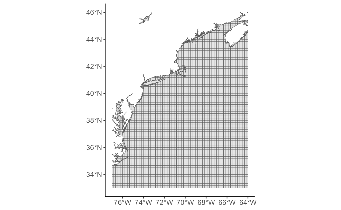
load_spatial(spat = FishSET::tenMNSQR, project = proj, name = "TenMNSQR")
#> Writing layer `scallopTenMNSQRSpatTable' to data source 
#>   `C:\Users\pcarvalho\AppData\Local\Temp\RtmpaASmG6/scallop/data/spat/scallopTenMNSQRSpatTable.geojson' using driver `GeoJSON'
#> Writing 5267 features with 9 fields and geometry type Polygon.
#> Writing layer `scallopTenMNSQRSpatTable20240807' to data source 
#>   `C:\Users\pcarvalho\AppData\Local\Temp\RtmpaASmG6/scallop/data/spat/scallopTenMNSQRSpatTable20240807.geojson' using driver `GeoJSON'
#> Writing 5267 features with 9 fields and geometry type Polygon.
#> Spatial table saved to project folder as scallopTenMNSQRSpatTable

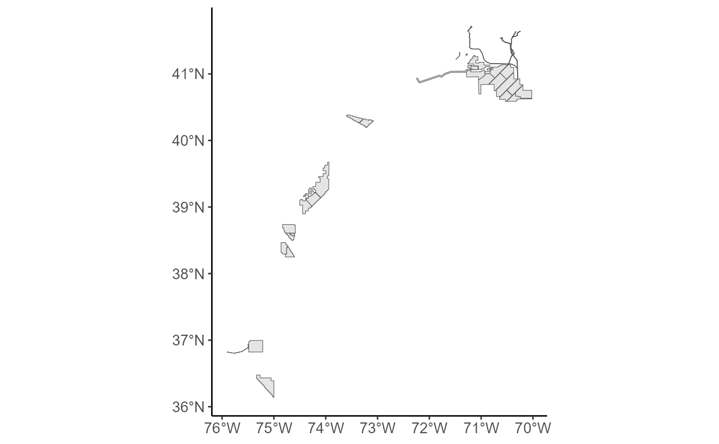
load_spatial(spat = FishSET::windLease, project = proj, name = "WindClose")
#> Writing layer `scallopWindCloseSpatTable' to data source 
#>   `C:\Users\pcarvalho\AppData\Local\Temp\RtmpaASmG6/scallop/data/spat/scallopWindCloseSpatTable.geojson' using driver `GeoJSON'
#> Writing 32 features with 1 fields and geometry type Multi Polygon.
#> Writing layer `scallopWindCloseSpatTable20240807' to data source 
#>   `C:\Users\pcarvalho\AppData\Local\Temp\RtmpaASmG6/scallop/data/spat/scallopWindCloseSpatTable20240807.geojson' using driver `GeoJSON'
#> Writing 32 features with 1 fields and geometry type Multi Polygon.
#> Spatial table saved to project folder as scallopWindCloseSpatTable

Assign the regulatory zones (scallopTenMNSQRSpatTable) and closure areas (scallopWindCloseSpatTable) to the working environment.

scallopTenMNSQRSpatTable <- table_view("scallopTenMNSQRSpatTable", proj)
#> Reading layer `scallopTenMNSQRSpatTable' from data source 
#>   `C:\Users\pcarvalho\AppData\Local\Temp\RtmpaASmG6\scallop\data\spat\scallopTenMNSQRSpatTable.geojson' 
#>   using driver `GeoJSON'
#> Simple feature collection with 5267 features and 9 fields
#> Geometry type: POLYGON
#> Dimension:     XY
#> Bounding box:  xmin: -77 ymin: 33 xmax: -64 ymax: 46.00139
#> Geodetic CRS:  NAD83
scallopWindCloseSpatTable <- table_view("scallopWindCloseSpatTable", proj)
#> Reading layer `scallopWindCloseSpatTable' from data source 
#>   `C:\Users\pcarvalho\AppData\Local\Temp\RtmpaASmG6\scallop\data\spat\scallopWindCloseSpatTable.geojson' 
#>   using driver `GeoJSON'
#> Simple feature collection with 32 features and 1 field
#> Geometry type: MULTIPOLYGON
#> Dimension:     XY
#> Bounding box:  xmin: -75.90347 ymin: 36.14111 xmax: -70.02155 ymax: 41.71859
#> Geodetic CRS:  WGS 84

Fleet assignment

Assign all observations to either “Access Area” or “Days at Sea” fleets.

fleet_tab <- 
  data.frame(
    condition = c('`Plan Code` == "SES" & `Program Code` == "SAA"',
                  '`Plan Code` == "SES" & `Program Code` == "SCA"'),
    fleet = c("Access Area", "Days at Sea"))

# save fleet table to FishSET DB
fleet_table(scallopMainDataTable, 
            project = proj,
            table = fleet_tab, save = TRUE)
#> Table saved to fishset_db database
#>                                        condition       fleet
#> 1 `Plan Code` == "SES" & `Program Code` == "SAA" Access Area
#> 2 `Plan Code` == "SES" & `Program Code` == "SCA" Days at Sea
# grab tab name
fleet_tab_name <- list_tables(proj, type = "fleet")
# create fleet column
scallopMainDataTable <- 
  fleet_assign(scallopMainDataTable, project = proj, 
               fleet_tab = fleet_tab_name)

Bin Gears

The data contain several types of fishing gear. For simplicity, the GEARCODE column is re-binned to include three categories: "DREDGE", "TRAWL-BOTTOM", and "OTHER".

scallopMainDataTable$GEARCODE_OLD <- scallopMainDataTable$GEARCODE
#Anything with "DREDGE" in the GEARCODE will be rebinned to "DREDGE" 
pat_match <- "*DREDGE*"
reg_pat <- glob2rx(pat_match)
scallopMainDataTable$GEARCODE[grep(reg_pat, scallopMainDataTable$GEARCODE)] <- 'DREDGE'
#Look at the GEARCODE NOW, there should be 'DREDGE', 'TRAWL-BOTTOM', and some funky stuff
table(scallopMainDataTable$GEARCODE)
#> 
#>       DREDGE        OTHER TRAWL-BOTTOM 
#>         9916            1           83
scallopMainDataTable$GEARCODE[!(scallopMainDataTable$GEARCODE %in% c('DREDGE','TRAWL-BOTTOM'))] <- 'OTHER'

Operating Profit

Calculate operating profit by subtracting 2020 trip costs from aggregated revenues in 2020 dollars.

scallopMainDataTable <- 
  scallopMainDataTable %>% 
  mutate(OPERATING_PROFIT_2020 = DOLLAR_ALL_SP_2020_OBSCURED - TRIP_COST_WINSOR_2020_DOL)

Summary Table

summary_stats(scallopMainDataTable, proj) %>% 
  pretty_tab_sb()

TRIPID	PERMIT.y	TRIP_LENGTH	port_lat	port_lon	previous_port_lat	previous_port_lon	TRIP_COST_WINSOR_2020_DOL	DDLAT	DDLON	ZoneID	LANDED_OBSCURED	DOLLAR_OBSCURED	DOLLAR_2020_OBSCURED	DOLLAR_ALL_SP_2020_OBSCURED	fleetAssignPlaceholder	OPERATING_PROFIT_2020	DATE_TRIP	GEARCODE	Plan Code	Program Code	fleet	GEARCODE_OLD
Min. : 6	Min. : 1	Min. : 0.15	Min. :37	Min. :-76	Min. :35	Min. :-77	Min. : 484	Min. :35	Min. :-76	Min. :357223	Min. : 22	Min. : 174	Min. : 204	Min. : 204	Min. :1	Min. : -12390	First: 2007-05-01	First: DREDGE	First: SES	First: SCA	First: Days at Sea	First: DREDGE-SCALLOP
Median :18836	Median :218	Median : 7.17	Median :42	Median :-71	Median :42	Median :-71	Median :12668	Median :40	Median :-73	Median :406712	Median :15639	Median :130938	Median :146722	Median : 148013	Median :1	Median : 134354	NA	NA	NA	NA	NA	NA
Mean :19076	Mean :236	Mean : 7.47	Mean :40	Mean :-73	Mean :40	Mean :-73	Mean :13886	Mean :40	Mean :-72	Mean :400612	Mean :14822	Mean :137458	Mean :151992	Mean : 156171	Mean :1	Mean : 142285	NA	NA	NA	NA	NA	NA
Max. :38503	Max. :456	Max. :24.58	Max. :42	Max. :-71	Max. :44	Max. :-70	Max. :30596	Max. :43	Max. :-66	Max. :427066	Max. :76507	Max. :648601	Max. :721698	Max. :2412282	Max. :1	Max. :2396500	NA	NA	NA	NA	NA	NA
NA’s: 0	NA’s: 0	NA’s: 0	NA’s: 0	NA’s: 0	NA’s: 18	NA’s: 18	NA’s: 0	NA’s: 0	NA’s: 0	NA’s: 5	NA’s: 0	NA’s: 0	NA’s: 0	NA’s: 0	NA’s: 0	NA’s: 0	NA’s: 0	NA’s: 0	NA’s: 0	NA’s: 0	NA’s: 0	NA’s: 0
Unique Obs: 10000	Unique Obs: 130	Unique Obs: 3923	Unique Obs: 6	Unique Obs: 6	Unique Obs: 41	Unique Obs: 41	Unique Obs: 9651	Unique Obs: 2039	Unique Obs: 2212	Unique Obs: 469	Unique Obs: 10000	Unique Obs: 10000	Unique Obs: 10000	Unique Obs: 10000	Unique Obs: 1	Unique Obs: 10000	Unique Obs: 3539	Unique Obs: 3	Unique Obs: 1	Unique Obs: 2	Unique Obs: 2	Unique Obs: 4
No. 0’s: 0	No. 0’s: 0	No. 0’s: 0	No. 0’s: 0	No. 0’s: 0	No. 0’s: NA	No. 0’s: NA	No. 0’s: 0	No. 0’s: 0	No. 0’s: 0	No. 0’s: NA	No. 0’s: 0	No. 0’s: 0	No. 0’s: 0	No. 0’s: 0	No. 0’s: 0	No. 0’s: 0	No. Empty: 0	No. Empty: 0	No. Empty: 0	No. Empty: 0	No. Empty: 0	No. Empty: 0

QAQC

NA Check

na_filter(scallopMainDataTable, 
          project = proj, 
          replace = FALSE, remove = FALSE, 
          rep.value = NA, over_write = FALSE)
#> The following columns contain NAs: previous_port_lat, previous_port_lon, ZoneID. Consider using na_filter to replace or remove NAs.

NaN Check

nan_filter(scallopMainDataTable, 
           project = proj, 
           replace = FALSE, remove = FALSE, 
           rep.value = NA, over_write = FALSE)
#> No NaNs found.

Unique Rows

unique_filter(scallopMainDataTable, project = proj, remove = FALSE)
#> Unique filter check for scallopMainDataTable dataset on 20240807 
#> Each row is a unique choice occurrence. No further action required.

Empty Variables

“Empty” variables contain all NAs.

empty_vars_filter(scallopMainDataTable, project = proj, remove = FALSE)
#> Empty vars check for scallopMainDataTable dataset on 20240807 
#> No empty variables identified.

Lon/Lat Format

degree(scallopMainDataTable, project = proj,
       lat = "DDLAT", lon = "DDLON", 
       latsign = NULL, lonsign = NULL,
       replace = FALSE)
#> Latitude and longitude variables in decimal degrees. No further action required.

Spatial QAQC

spat_qaqc_out <- spatial_qaqc(dat = scallopMainDataTable, 
                              project = proj,
                              spat = scallopTenMNSQRSpatTable, 
                              lon.dat = "DDLON", 
                              lat.dat = "DDLAT")
#> Warning: Spatial reference EPSG codes for the spatial and primary datasets do
#> not match. The detected projection in the spatial file will be used unless epsg
#> is specified.
#> Warning: 10 observations (0.1%) occur on land.
#> Warning: 35 observations (0.4%) occur on boundary line between regulatory zones.
#> 10 observations (0.1%) occur on land.
#> 35 observations (0.4%) occur on boundary line between regulatory zones.

spat_qaqc_out$dataset <- NULL # drop dataset

spat_qaqc_out$spatial_summary %>%
  pretty_lab(cols = "n") %>%
  pretty_tab()

YEAR	n	EXPECTED_LOC	ON_LAND	ON_ZONE_BOUNDARY	perc
2007	773	766	2	5	7.73
2008	822	821	0	1	8.22
2009	861	858	1	2	8.61
2010	864	862	1	1	8.64
2011	818	814	0	4	8.18
2012	784	783	0	1	7.84
2013	603	599	1	3	6.03
2014	523	520	1	2	5.23
2015	601	596	0	5	6.01
2016	682	680	0	2	6.82
2017	788	785	0	3	7.88
2018	896	891	0	5	8.96
2019	985	980	4	1	9.85

spat_qaqc_out[2:4]
#> $land_plot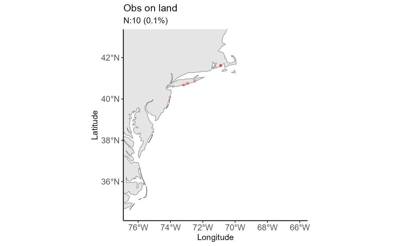

#> 
#> $boundary_plot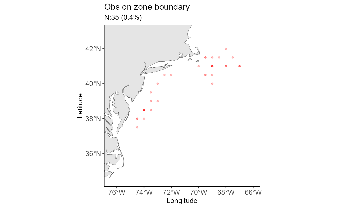

#> 
#> $expected_plot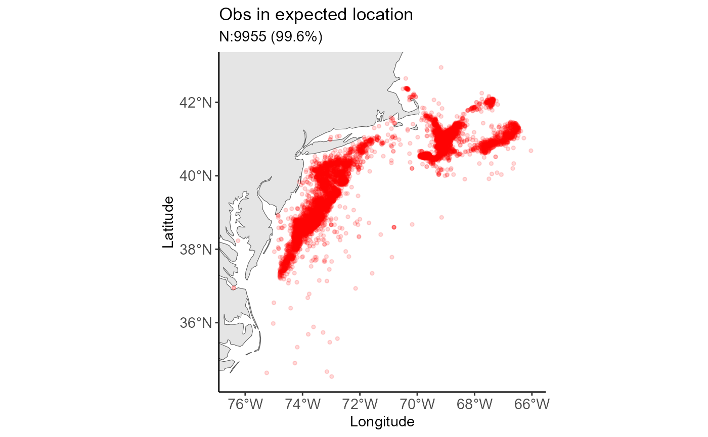

Data Creation

Landing Year

scallopMainDataTable <- 
  scallopMainDataTable %>% 
  mutate(DB_LANDING_YEAR = as.numeric(format(date_parser(DATE_TRIP), "%Y")))

Finagle LANDED_OBSCURED to Thousands of Pounds

scallopMainDataTable$LANDED_OBSCURED <- scallopMainDataTable$LANDED_OBSCURED / 1000

CPUE

Create CPUE variable using TRIP_LENGTH and LANDED_OBSCURED. Filter out any infinite values.

scallopMainDataTable <- 
  cpue(scallopMainDataTable, proj,
       xWeight = "LANDED_OBSCURED",
       xTime = "TRIP_LENGTH", 
       name = "CPUE")
#> Warning: xWeight must a measurement of mass. CPUE calculated.
#> Warning: xTime should be a measurement of time. Use the create_duration
#> function. CPUE calculated.

scallopMainDataTable <- 
  scallopMainDataTable %>% 
  filter(!is.infinite(CPUE))

CPUE Percent Rank

Add a percent rank column to filter outliers.

outlier_table(scallopMainDataTable, proj, x = "CPUE") %>% 
  pretty_lab() %>% 
  pretty_tab()

Vector	outlier_check	N	mean	median	SD	min	max	NAs	skew
CPUE	None	10,000	2.01	1.95	2	0.01	149.98	0	45.53
CPUE	5_95_quant	9,000	1.95	1.95	0.73	0.49	3.47	0	0.01
CPUE	25_75_quant	5,000	1.95	1.95	0.35	1.31	2.57	0	-0.03
CPUE	mean_2SD	9,973	1.96	1.95	0.9	0.01	5.79	0	0.23
CPUE	mean_3SD	9,984	1.96	1.95	0.91	0.01	7.92	0	0.4
CPUE	median_2SD	9,973	1.96	1.95	0.9	0.01	5.79	0	0.23
CPUE	median_3SD	9,984	1.96	1.95	0.91	0.01	7.92	0	0.4

scallopMainDataTable <- 
  scallopMainDataTable %>% 
  mutate(CPUE_p = percent_rank(CPUE))

VPUE

Same as above but with revenue instead of meat pounds.

scallopMainDataTable <- 
  cpue(scallopMainDataTable, proj,
       xWeight = "DOLLAR_OBSCURED",
       xTime = "TRIP_LENGTH", 
       name = "VPUE")
#> Warning: xWeight must a measurement of mass. CPUE calculated.
#> Warning: xTime should be a measurement of time. Use the create_duration
#> function. CPUE calculated.

scallopMainDataTable <- 
  scallopMainDataTable %>% 
  filter(!is.infinite(VPUE))

VPUE Percent Rank

Add a percent rank column to filter outliers.

outlier_table(scallopMainDataTable, proj, x = "VPUE") %>% 
  pretty_lab() %>% 
  pretty_tab()

Vector	outlier_check	N	mean	median	SD	min	max	NAs	skew
VPUE	None	10,000	18,675.14	17,691.99	15,505.59	92.36	933,919.8	0	26.74
VPUE	5_95_quant	9,000	18,026.09	17,691.99	7,670.15	4,199.84	35,185.46	0	0.2
VPUE	25_75_quant	5,000	17,704.31	17,691.99	3,802.8	11,073.26	24,564.41	0	0.02
VPUE	mean_2SD	9,947	18,203.17	17,639.59	9,281	92.36	49,607.4	0	0.39
VPUE	mean_3SD	9,978	18,315.2	17,670.87	9,483.24	92.36	64,302.48	0	0.51
VPUE	median_2SD	9,944	18,193.81	17,635.59	9,266.73	92.36	48,637.5	0	0.39
VPUE	median_3SD	9,977	18,310.59	17,670.19	9,472.53	92.36	59,843.36	0	0.5

scallopMainDataTable <- 
  scallopMainDataTable %>% 
  mutate(VPUE_p = percent_rank(VPUE))

Fleet Tabulation

scallopMainDataTable %>% 
  count(fleet) %>% 
  mutate(perc = round(n/sum(n) * 100, 1)) %>% 
  pretty_lab(cols = "n") %>% 
  pretty_tab()

fleet	n	perc
Access Area	5,678	56.8
Days at Sea	4,322	43.2

Zone Assignment

Assign each observation to a regulatory zone.

scallopMainDataTable <- 
  assignment_column(scallopMainDataTable, project = proj,
                    spat = scallopTenMNSQRSpatTable, 
                    lon.dat = "DDLON",
                    lat.dat = "DDLAT", 
                    cat = "TEN_ID",
                    name = "ZONE_ID",
                    closest.pt = FALSE,
                    hull.polygon = FALSE)
#> Warning: Projection does not match. The detected projection in the spatial file
#> will be used unless epsg is specified.
#> Warning: At least one observation assigned to multiple regulatory zones.
#> Assigning observations to nearest polygon.

Closure Area Assignment

Assign each observation to a closure area. An observation will have an NA if it does not occur within a closure area.

scallopMainDataTable <- 
  assignment_column(scallopMainDataTable, project = proj,
                    spat = scallopWindCloseSpatTable, 
                    lon.dat = "DDLON",
                    lat.dat = "DDLAT", 
                    cat = "NAME",
                    name = "closeID",
                    closest.pt = FALSE,
                    hull.polygon = FALSE) 

scallopMainDataTable <- 
  scallopMainDataTable %>% 
  mutate(in_closure = !is.na(closeID))

62 observations (0.62%) occurred inside a closure area.

agg_helper(scallopMainDataTable, 
           value = "in_closure", 
           count = TRUE, 
           fun = NULL) %>% 
  pivot_wider(names_from = "in_closure", values_from = "n") %>% 
  rename("Outside Closure(s)" = "FALSE", "Inside Closure(s)" = "TRUE") %>% 
  pretty_lab() %>% 
  pretty_tab()

Outside Closure(s)	Inside Closure(s)
9,938	62

Observations inside/outside closures by fleet.

agg_helper(scallopMainDataTable, group = "fleet", 
            value = "in_closure", count = TRUE, fun = NULL) %>% 
  pivot_wider(names_from = "in_closure", values_from = "n") %>% 
  rename("Outside Closure(s)" = "FALSE", "Inside Closure(s)" = "TRUE") %>% 
  pretty_lab() %>% 
  pretty_tab()

fleet	Outside Closure(s)	Inside Closure(s)
Access Area	5,668	10
Days at Sea	4,270	52

Observations inside/outside closures by year.

agg_helper(scallopMainDataTable, value = "in_closure", 
            group = "DB_LANDING_YEAR", 
            count = TRUE, fun = NULL) %>% 
  pivot_wider(names_from = "in_closure", values_from = "n",
              values_fill = 0) %>% 
  arrange(DB_LANDING_YEAR) %>% 
  rename("Outside closure(s)" = "FALSE", "Inside closure(s)" = "TRUE") %>% 
  pretty_lab(ignore = "DB_LANDING_YEAR") %>% 
  pretty_tab()

DB_LANDING_YEAR	Outside closure(s)	Inside closure(s)
2007	773	0
2008	814	8
2009	855	6
2010	855	9
2011	807	11
2012	780	4
2013	599	4
2014	521	2
2015	598	3
2016	677	5
2017	785	3
2018	894	2
2019	980	5

Observations inside/outside closures by year and fleet.

agg_helper(scallopMainDataTable, value = "in_closure", 
            group = c("DB_LANDING_YEAR", "fleet"), 
            count = TRUE, fun = NULL) %>% 
  pivot_wider(names_from = "in_closure", values_from = "n",
              values_fill = 0) %>% 
  arrange(DB_LANDING_YEAR) %>% 
  rename("Outside closure(s)" = "FALSE", "Inside closure(s)" = "TRUE") %>% 
  pretty_lab(ignore = "DB_LANDING_YEAR") %>% 
  pretty_tab_sb(width = "60%") 

DB_LANDING_YEAR	fleet	Outside closure(s)	Inside closure(s)
2007	Access Area	423	0
2007	Days at Sea	350	0
2008	Access Area	471	0
2008	Days at Sea	343	8
2009	Access Area	479	2
2009	Days at Sea	376	4
2010	Access Area	454	4
2010	Days at Sea	401	5
2011	Access Area	500	1
2011	Days at Sea	307	10
2012	Access Area	438	0
2012	Days at Sea	342	4
2013	Days at Sea	353	4
2013	Access Area	246	0
2014	Days at Sea	348	2
2014	Access Area	173	0
2015	Access Area	304	0
2015	Days at Sea	294	3
2016	Access Area	354	2
2016	Days at Sea	323	3
2017	Access Area	464	0
2017	Days at Sea	321	3
2018	Access Area	624	0
2018	Days at Sea	270	2
2019	Access Area	738	1
2019	Days at Sea	242	4

Zone Summary

Frequency

The number of observations by zone.

zone_out <- zone_summary(scallopMainDataTable, project = proj,
                         spat = scallopTenMNSQRSpatTable,
                         zone.dat = "ZONE_ID",
                         zone.spat = "TEN_ID",
                         output = "tab_plot",
                         count = TRUE,
                         breaks = NULL, n.breaks = 10,
                         na.rm = TRUE)
#> A line object has been specified, but lines is not in the mode
#> Adding lines to the mode...

zone_out$plot

zone_out$table %>%
  pretty_lab(cols = "n") %>%
  pretty_tab_sb(width = "40%")

ZONE_ID	n
416965	265
387332	260
387331	231
387322	211
406932	194
387314	193
406926	192
387446	164
406915	151
387323	148
387436	146
387313	141
406925	140
406916	137
387445	135
416966	131
416862	122
387455	119
416861	119
387465	114
387333	109
397364	107
387426	96
397315	96
406933	96
397213	94
397232	91
397363	82
397231	80
397355	80
397365	80
406811	80
406936	80
416662	80
416944	79
387341	76
406942	76
416852	75
406935	74
387456	68
397241	68
416955	67
387435	66
397346	65
397325	63
406931	62
416661	60
406944	59
407364	59
387324	58
387342	56
407242	56
426764	56
416843	55
377433	54
397356	54
406715	54
407262	53
407365	52
406714	51
377424	50
416653	50
387312	49
387315	49
387321	49
397354	49
407263	48
407254	47
397212	46
406821	46
406943	46
416851	45
397223	44
406723	44
387425	43
397335	43
406945	40
377423	39
407355	39
397314	38
397366	38
407356	38
407366	37
397214	36
397326	36
397345	36
406713	36
407244	36
397362	35
407241	35
377443	34
406716	34
407243	34
407261	34
377442	33
406722	33
407121	33
397316	32
416643	32
416714	32
377414	31
387311	31
397336	31
406611	31
407253	31
416842	31
416853	31
407251	30
377415	29
397211	29
397242	29
407112	29
407363	29
397344	28
416954	28
397353	27
407113	27
416652	27
416713	27
387466	25
407131	25
407252	25
407354	23
416933	23
416945	23
387464	22
416642	22
416934	22
426763	22
406712	21
407245	21
416844	21
377432	20
397222	20
407346	20
416651	20
406724	19
406831	19
407345	19
416863	19
397251	18
397343	18
406812	18
416654	18
416765	18
407264	17
416816	17
416956	17
416964	17
397221	16
397324	16
406832	16
407226	16
416663	16
397334	15
406822	15
377452	14
397313	14
406733	14
407234	14
387334	13
416932	13
377413	12
377425	12
377434	12
387325	12
397352	12
397361	12
406732	12
406826	12
406965	11
407111	11
407122	11
427044	11
387416	10
406721	10
406841	10
407225	10
397333	9
407115	9
407236	9
407255	9
407256	9
427045	9
387351	8
397342	8
406833	8
407246	8
416766	8
417031	8
417164	8
427065	8
397224	7
397312	7
407114	7
407235	7
407353	7
416711	7
416834	7
406813	6
406934	6
416756	6
416826	6
416845	6
416854	6
377323	5
377422	5
387335	5
387336	5
387434	5
387463	5
406814	5
406815	5
406924	5
406954	5
407141	5
407232	5
407343	5
407362	5
416641	5
416712	5
416825	5
426765	5
427056	5
387032	4
387362	4
387432	4
406835	4
406861	4
406914	4
407132	4
407352	4
416721	4
417061	4
377416	3
377453	3
387242	3
387352	3
387363	3
387411	3
387452	3
397323	3
397351	3
397426	3
397465	3
406612	3
406711	3
406725	3
406816	3
406834	3
406946	3
406952	3
407055	3
407151	3
407266	3
407344	3
416943	3
417042	3
417062	3
427066	3
367322	2
367614	2
377325	2
377335	2
377435	2
377444	2
377464	2
387226	2
387241	2
387246	2
387326	2
387354	2
387355	2
387365	2
387415	2
387422	2
387444	2
387454	2
387462	2
397233	2
397234	2
397261	2
397311	2
397322	2
397332	2
397456	2
397466	2
406613	2
406621	2
406734	2
406735	2
406742	2
406862	2
406941	2
406955	2
407013	2
407021	2
407032	2
407041	2
407142	2
407216	2
407221	2
407233	2
407265	2
407316	2
407335	2
407336	2
407361	2
416722	2
416744	2
416755	2
416761	2
416824	2
416833	2
416864	2
416912	2
416922	2
416935	2
416953	2
416961	2
416963	2
417055	2
417262	2
426762	2
0	1
347231	1
347336	1
347415	1
347535	1
357232	1
357313	1
357322	1
357325	1
357346	1
357445	1
357516	1
367216	1
367444	1
367536	1
377021	1
377143	1
377214	1
377224	1
377231	1
377312	1
377321	1
377322	1
377332	1
377346	1
377364	1
377366	1
377411	1
377426	1
377445	1
377465	1
386916	1
387025	1
387122	1
387145	1
387211	1
387212	1
387214	1
387225	1
387231	1
387232	1
387233	1
387236	1
387244	1
387252	1
387344	1
387345	1
387353	1
387361	1
387366	1
387413	1
387414	1
387424	1
387433	1
387461	1
387655	1
396714	1
396814	1
396916	1
397225	1
397246	1
397262	1
397263	1
397265	1
397321	1
397331	1
397446	1
397463	1
397464	1
406623	1
406626	1
406643	1
406652	1
406731	1
406744	1
406764	1
406765	1
406766	1
406852	1
406923	1
406966	1
407011	1
407012	1
407015	1
407035	1
407045	1
407116	1
407123	1
407133	1
407134	1
407135	1
407163	1
407215	1
407223	1
407224	1
407231	1
407325	1
407326	1
407333	1
407342	1
407466	1
416644	1
416664	1
416665	1
416715	1
416724	1
416734	1
416742	1
416746	1
416762	1
416764	1
416831	1
416835	1
416841	1
416856	1
416865	1
416866	1
416915	1
416916	1
416924	1
416931	1
416942	1
416952	1
416962	1
417041	1
417046	1
417051	1
417145	1
417146	1
417154	1
417161	1
417162	1
417163	1
417165	1
417166	1
417366	1
426752	1
426761	1
426915	1
426964	1
427034	1

Percent of observations by zone.

zone_out <- 
  zone_summary(scallopMainDataTable,
               project = proj,
               spat = scallopTenMNSQRSpatTable,
               zone.dat = "ZONE_ID",
               zone.spat = "TEN_ID",
               output = "tab_plot",
               count = TRUE, fun = "percent",
               breaks = c(seq(.2, .5, .1), seq(1, 2, .5)), 
               na.rm = TRUE)
#> A line object has been specified, but lines is not in the mode
#> Adding lines to the mode...

zone_out$plot

zone_out$table %>% 
  pretty_lab(ignore = "ZONE_ID") %>% 
  pretty_tab_sb(width = "40%")

ZONE_ID	n	perc
416965	265	2.65
387332	260	2.6
387331	231	2.31
387322	211	2.11
406932	194	1.94
387314	193	1.93
406926	192	1.92
387446	164	1.64
406915	151	1.51
387323	148	1.48
387436	146	1.46
387313	141	1.41
406925	140	1.4
406916	137	1.37
387445	135	1.35
416966	131	1.31
416862	122	1.22
387455	119	1.19
416861	119	1.19
387465	114	1.14
387333	109	1.09
397364	107	1.07
387426	96	0.96
397315	96	0.96
406933	96	0.96
397213	94	0.94
397232	91	0.91
397363	82	0.82
397231	80	0.8
397355	80	0.8
397365	80	0.8
406811	80	0.8
406936	80	0.8
416662	80	0.8
416944	79	0.79
387341	76	0.76
406942	76	0.76
416852	75	0.75
406935	74	0.74
387456	68	0.68
397241	68	0.68
416955	67	0.67
387435	66	0.66
397346	65	0.65
397325	63	0.63
406931	62	0.62
416661	60	0.6
406944	59	0.59
407364	59	0.59
387324	58	0.58
387342	56	0.56
407242	56	0.56
426764	56	0.56
416843	55	0.55
377433	54	0.54
397356	54	0.54
406715	54	0.54
407262	53	0.53
407365	52	0.52
406714	51	0.51
377424	50	0.5
416653	50	0.5
387312	49	0.49
387315	49	0.49
387321	49	0.49
397354	49	0.49
407263	48	0.48
407254	47	0.47
397212	46	0.46
406821	46	0.46
406943	46	0.46
416851	45	0.45
397223	44	0.44
406723	44	0.44
387425	43	0.43
397335	43	0.43
406945	40	0.4
377423	39	0.39
407355	39	0.39
397314	38	0.38
397366	38	0.38
407356	38	0.38
407366	37	0.37
397214	36	0.36
397326	36	0.36
397345	36	0.36
406713	36	0.36
407244	36	0.36
397362	35	0.35
407241	35	0.35
377443	34	0.34
406716	34	0.34
407243	34	0.34
407261	34	0.34
377442	33	0.33
406722	33	0.33
407121	33	0.33
397316	32	0.32
416643	32	0.32
416714	32	0.32
377414	31	0.31
387311	31	0.31
397336	31	0.31
406611	31	0.31
407253	31	0.31
416842	31	0.31
416853	31	0.31
407251	30	0.3
377415	29	0.29
397211	29	0.29
397242	29	0.29
407112	29	0.29
407363	29	0.29
397344	28	0.28
416954	28	0.28
397353	27	0.27
407113	27	0.27
416652	27	0.27
416713	27	0.27
387466	25	0.25
407131	25	0.25
407252	25	0.25
407354	23	0.23
416933	23	0.23
416945	23	0.23
387464	22	0.22
416642	22	0.22
416934	22	0.22
426763	22	0.22
406712	21	0.21
407245	21	0.21
416844	21	0.21
377432	20	0.2
397222	20	0.2
407346	20	0.2
416651	20	0.2
406724	19	0.19
406831	19	0.19
407345	19	0.19
416863	19	0.19
397251	18	0.18
397343	18	0.18
406812	18	0.18
416654	18	0.18
416765	18	0.18
407264	17	0.17
416816	17	0.17
416956	17	0.17
416964	17	0.17
397221	16	0.16
397324	16	0.16
406832	16	0.16
407226	16	0.16
416663	16	0.16
397334	15	0.15
406822	15	0.15
377452	14	0.14
397313	14	0.14
406733	14	0.14
407234	14	0.14
387334	13	0.13
416932	13	0.13
377413	12	0.12
377425	12	0.12
377434	12	0.12
387325	12	0.12
397352	12	0.12
397361	12	0.12
406732	12	0.12
406826	12	0.12
406965	11	0.11
407111	11	0.11
407122	11	0.11
427044	11	0.11
387416	10	0.1
406721	10	0.1
406841	10	0.1
407225	10	0.1
397333	9	0.09
407115	9	0.09
407236	9	0.09
407255	9	0.09
407256	9	0.09
427045	9	0.09
387351	8	0.08
397342	8	0.08
406833	8	0.08
407246	8	0.08
416766	8	0.08
417031	8	0.08
417164	8	0.08
427065	8	0.08
397224	7	0.07
397312	7	0.07
407114	7	0.07
407235	7	0.07
407353	7	0.07
416711	7	0.07
416834	7	0.07
406813	6	0.06
406934	6	0.06
416756	6	0.06
416826	6	0.06
416845	6	0.06
416854	6	0.06
377323	5	0.05
377422	5	0.05
387335	5	0.05
387336	5	0.05
387434	5	0.05
387463	5	0.05
406814	5	0.05
406815	5	0.05
406924	5	0.05
406954	5	0.05
407141	5	0.05
407232	5	0.05
407343	5	0.05
407362	5	0.05
416641	5	0.05
416712	5	0.05
416825	5	0.05
426765	5	0.05
427056	5	0.05
387032	4	0.04
387362	4	0.04
387432	4	0.04
406835	4	0.04
406861	4	0.04
406914	4	0.04
407132	4	0.04
407352	4	0.04
416721	4	0.04
417061	4	0.04
377416	3	0.03
377453	3	0.03
387242	3	0.03
387352	3	0.03
387363	3	0.03
387411	3	0.03
387452	3	0.03
397323	3	0.03
397351	3	0.03
397426	3	0.03
397465	3	0.03
406612	3	0.03
406711	3	0.03
406725	3	0.03
406816	3	0.03
406834	3	0.03
406946	3	0.03
406952	3	0.03
407055	3	0.03
407151	3	0.03
407266	3	0.03
407344	3	0.03
416943	3	0.03
417042	3	0.03
417062	3	0.03
427066	3	0.03
367322	2	0.02
367614	2	0.02
377325	2	0.02
377335	2	0.02
377435	2	0.02
377444	2	0.02
377464	2	0.02
387226	2	0.02
387241	2	0.02
387246	2	0.02
387326	2	0.02
387354	2	0.02
387355	2	0.02
387365	2	0.02
387415	2	0.02
387422	2	0.02
387444	2	0.02
387454	2	0.02
387462	2	0.02
397233	2	0.02
397234	2	0.02
397261	2	0.02
397311	2	0.02
397322	2	0.02
397332	2	0.02
397456	2	0.02
397466	2	0.02
406613	2	0.02
406621	2	0.02
406734	2	0.02
406735	2	0.02
406742	2	0.02
406862	2	0.02
406941	2	0.02
406955	2	0.02
407013	2	0.02
407021	2	0.02
407032	2	0.02
407041	2	0.02
407142	2	0.02
407216	2	0.02
407221	2	0.02
407233	2	0.02
407265	2	0.02
407316	2	0.02
407335	2	0.02
407336	2	0.02
407361	2	0.02
416722	2	0.02
416744	2	0.02
416755	2	0.02
416761	2	0.02
416824	2	0.02
416833	2	0.02
416864	2	0.02
416912	2	0.02
416922	2	0.02
416935	2	0.02
416953	2	0.02
416961	2	0.02
416963	2	0.02
417055	2	0.02
417262	2	0.02
426762	2	0.02
0	1	0.01
347231	1	0.01
347336	1	0.01
347415	1	0.01
347535	1	0.01
357232	1	0.01
357313	1	0.01
357322	1	0.01
357325	1	0.01
357346	1	0.01
357445	1	0.01
357516	1	0.01
367216	1	0.01
367444	1	0.01
367536	1	0.01
377021	1	0.01
377143	1	0.01
377214	1	0.01
377224	1	0.01
377231	1	0.01
377312	1	0.01
377321	1	0.01
377322	1	0.01
377332	1	0.01
377346	1	0.01
377364	1	0.01
377366	1	0.01
377411	1	0.01
377426	1	0.01
377445	1	0.01
377465	1	0.01
386916	1	0.01
387025	1	0.01
387122	1	0.01
387145	1	0.01
387211	1	0.01
387212	1	0.01
387214	1	0.01
387225	1	0.01
387231	1	0.01
387232	1	0.01
387233	1	0.01
387236	1	0.01
387244	1	0.01
387252	1	0.01
387344	1	0.01
387345	1	0.01
387353	1	0.01
387361	1	0.01
387366	1	0.01
387413	1	0.01
387414	1	0.01
387424	1	0.01
387433	1	0.01
387461	1	0.01
387655	1	0.01
396714	1	0.01
396814	1	0.01
396916	1	0.01
397225	1	0.01
397246	1	0.01
397262	1	0.01
397263	1	0.01
397265	1	0.01
397321	1	0.01
397331	1	0.01
397446	1	0.01
397463	1	0.01
397464	1	0.01
406623	1	0.01
406626	1	0.01
406643	1	0.01
406652	1	0.01
406731	1	0.01
406744	1	0.01
406764	1	0.01
406765	1	0.01
406766	1	0.01
406852	1	0.01
406923	1	0.01
406966	1	0.01
407011	1	0.01
407012	1	0.01
407015	1	0.01
407035	1	0.01
407045	1	0.01
407116	1	0.01
407123	1	0.01
407133	1	0.01
407134	1	0.01
407135	1	0.01
407163	1	0.01
407215	1	0.01
407223	1	0.01
407224	1	0.01
407231	1	0.01
407325	1	0.01
407326	1	0.01
407333	1	0.01
407342	1	0.01
407466	1	0.01
416644	1	0.01
416664	1	0.01
416665	1	0.01
416715	1	0.01
416724	1	0.01
416734	1	0.01
416742	1	0.01
416746	1	0.01
416762	1	0.01
416764	1	0.01
416831	1	0.01
416835	1	0.01
416841	1	0.01
416856	1	0.01
416865	1	0.01
416866	1	0.01
416915	1	0.01
416916	1	0.01
416924	1	0.01
416931	1	0.01
416942	1	0.01
416952	1	0.01
416962	1	0.01
417041	1	0.01
417046	1	0.01
417051	1	0.01
417145	1	0.01
417146	1	0.01
417154	1	0.01
417161	1	0.01
417162	1	0.01
417163	1	0.01
417165	1	0.01
417166	1	0.01
417366	1	0.01
426752	1	0.01
426761	1	0.01
426915	1	0.01
426964	1	0.01
427034	1	0.01

Zone frequency (Access Area fleet).

zone_out <- 
  scallopMainDataTable %>% 
    filter(fleet == "Access Area") %>% 
    zone_summary(project = proj,
                 spat = scallopTenMNSQRSpatTable, 
                 zone.dat = "ZONE_ID",
                 zone.spat = "TEN_ID",
                 output = "tab_plot",
                 count = TRUE,
                 breaks = NULL, n.breaks = 10, 
                 na.rm = TRUE)
#> A line object has been specified, but lines is not in the mode
#> Adding lines to the mode...

zone_out$plot

zone_out$table %>% 
  pretty_lab(cols = "n") %>% 
  pretty_tab_sb(width = "40%")

ZONE_ID	n
387332	258
387331	229
387322	208
406932	194
387314	192
406926	191
387446	163
387323	147
387436	145
406925	140
387445	133
416862	121
387455	117
387313	116
387465	109
387333	106
416861	106
387426	96
406933	96
397364	91
416662	80
406936	77
406942	76
387341	75
416852	75
397365	74
406935	73
387456	68
397355	68
387435	66
406931	62
397346	60
416661	60
406944	59
387324	57
397241	57
416843	55
377433	54
387342	54
397356	51
416653	49
387321	48
387315	47
377424	46
406943	46
416851	45
387425	42
377423	39
406945	39
416966	36
377442	33
377443	33
397366	32
416643	32
377414	31
416842	31
416853	31
416652	27
377415	26
387464	22
387466	22
406811	22
416642	22
397242	21
377432	20
416651	20
416863	19
406812	15
416654	15
416663	15
397251	14
406821	13
416765	13
377413	12
377434	12
387325	12
387334	12
377452	11
397363	11
377425	10
397345	9
416844	9
416956	9
397354	8
416766	8
387311	7
387351	7
406934	6
387312	5
387335	5
387463	5
406831	5
406954	5
416641	5
416854	5
417031	5
377422	4
387032	4
387336	4
387362	4
387432	4
397334	4
406861	4
406924	4
416756	4
377416	3
387242	3
387434	3
387452	3
397232	3
397333	3
397342	3
406813	3
406915	3
406946	3
406952	3
407246	3
407255	3
407343	3
416945	3
416965	3
417042	3
367322	2
367614	2
377323	2
377435	2
377444	2
377453	2
387226	2
387241	2
387246	2
387352	2
387365	2
387411	2
387415	2
387422	2
387454	2
387462	2
397313	2
397322	2
397362	2
397426	2
397456	2
406613	2
406735	2
406862	2
406941	2
406955	2
407032	2
407355	2
416755	2
416864	2
416943	2
416953	2
416961	2
417262	2
347415	1
347535	1
357313	1
357322	1
357346	1
357445	1
357516	1
367216	1
367444	1
367536	1
377021	1
377224	1
377312	1
377332	1
377346	1
377364	1
377366	1
377411	1
377426	1
377445	1
377465	1
387122	1
387145	1
387211	1
387212	1
387214	1
387225	1
387232	1
387233	1
387236	1
387244	1
387326	1
387345	1
387353	1
387355	1
387361	1
387366	1
387413	1
387414	1
387416	1
387424	1
387433	1
387444	1
387461	1
387655	1
396916	1
397211	1
397212	1
397231	1
397234	1
397261	1
397262	1
397263	1
397265	1
397312	1
397314	1
397315	1
397321	1
397324	1
397326	1
397331	1
397332	1
397336	1
397343	1
397353	1
397446	1
397464	1
397465	1
397466	1
406611	1
406643	1
406652	1
406712	1
406714	1
406716	1
406724	1
406742	1
406816	1
406822	1
406835	1
406852	1
406916	1
406923	1
407035	1
407045	1
407111	1
407113	1
407121	1
407251	1
407326	1
407336	1
407342	1
407344	1
407345	1
407362	1
407363	1
416644	1
416664	1
416715	1
416722	1
416742	1
416744	1
416746	1
416856	1
416866	1
416931	1
416932	1
416933	1
416935	1
416952	1
416955	1
416963	1
417051	1
417146	1
426761	1

Zone frequency (Days at Sea fleet).

zone_out <- 
  scallopMainDataTable %>% 
    filter(fleet == "Days at Sea") %>% 
    zone_summary(project = proj,
                 spat = scallopTenMNSQRSpatTable,
                 zone.dat = "ZONE_ID",
                 zone.spat = "TEN_ID",
                 output = "tab_plot",
                 count = TRUE,
                 breaks = NULL, n.breaks = 10, 
                 na.rm = TRUE)
#> A line object has been specified, but lines is not in the mode
#> Adding lines to the mode...

zone_out$plot

zone_out$table %>% 
  pretty_lab(cols = "n") %>% 
  pretty_tab_sb(width = "40%")

ZONE_ID	n
416965	262
406915	148
406916	136
397315	95
416966	95
397213	94
397232	88
397231	79
416944	79
397363	71
416955	66
397325	63
407364	59
406811	58
407242	56
426764	56
406715	54
407262	53
407365	52
406714	50
407263	48
407254	47
397212	45
387312	44
397223	44
406723	44
397335	43
397354	41
407356	38
397314	37
407355	37
407366	37
397214	36
406713	36
407244	36
397326	35
407241	35
407243	34
407261	34
397362	33
406716	33
406722	33
406821	33
397316	32
407121	32
416714	32
407253	31
397336	30
406611	30
407112	29
407251	29
397211	28
397344	28
407363	28
416954	28
397345	27
416713	27
397353	26
407113	26
387313	25
407131	25
407252	25
387311	24
407354	23
416933	22
416934	22
426763	22
407245	21
397222	20
406712	20
407346	20
416945	20
406724	18
407345	18
397343	17
407264	17
416816	17
416964	17
397221	16
397364	16
406832	16
407226	16
397324	15
406733	14
406822	14
406831	14
407234	14
416861	13
397313	12
397352	12
397355	12
397361	12
406732	12
406826	12
416844	12
416932	12
397241	11
397334	11
406965	11
407122	11
427044	11
406721	10
406841	10
407111	10
407225	10
387416	9
407115	9
407236	9
407256	9
427045	9
397242	8
406833	8
416956	8
417164	8
427065	8
397224	7
407114	7
407235	7
407353	7
416711	7
416834	7
397312	6
397333	6
397365	6
397366	6
407255	6
416826	6
416845	6
387465	5
397342	5
397346	5
406814	5
406815	5
407141	5
407232	5
407246	5
416712	5
416765	5
416825	5
426765	5
427056	5
377424	4
397251	4
406914	4
407132	4
407352	4
407362	4
416721	4
417061	4
377323	3
377415	3
377452	3
387322	3
387333	3
387363	3
387466	3
397323	3
397351	3
397356	3
406612	3
406711	3
406725	3
406812	3
406813	3
406834	3
406835	3
406936	3
407055	3
407151	3
407266	3
416654	3
417031	3
417062	3
427066	3
377325	2
377335	2
377425	2
377464	2
387315	2
387331	2
387332	2
387342	2
387354	2
387434	2
387445	2
387455	2
397233	2
397311	2
397465	2
406621	2
406734	2
406816	2
407013	2
407021	2
407041	2
407142	2
407216	2
407221	2
407233	2
407265	2
407316	2
407335	2
407343	2
407344	2
407361	2
416756	2
416761	2
416824	2
416833	2
416912	2
416922	2
417055	2
426762	2
0	1
347231	1
347336	1
357232	1
357325	1
377143	1
377214	1
377231	1
377321	1
377322	1
377422	1
377443	1
377453	1
386916	1
387025	1
387231	1
387252	1
387314	1
387321	1
387323	1
387324	1
387326	1
387334	1
387336	1
387341	1
387344	1
387351	1
387352	1
387355	1
387411	1
387425	1
387436	1
387444	1
387446	1
396714	1
396814	1
397225	1
397234	1
397246	1
397261	1
397332	1
397426	1
397463	1
397466	1
406623	1
406626	1
406731	1
406742	1
406744	1
406764	1
406765	1
406766	1
406924	1
406926	1
406935	1
406945	1
406966	1
407011	1
407012	1
407015	1
407116	1
407123	1
407133	1
407134	1
407135	1
407163	1
407215	1
407223	1
407224	1
407231	1
407325	1
407333	1
407336	1
407466	1
416653	1
416663	1
416665	1
416722	1
416724	1
416734	1
416744	1
416762	1
416764	1
416831	1
416835	1
416841	1
416854	1
416862	1
416865	1
416915	1
416916	1
416924	1
416935	1
416942	1
416943	1
416962	1
416963	1
417041	1
417046	1
417145	1
417154	1
417161	1
417162	1
417163	1
417165	1
417166	1
417366	1
426752	1
426915	1
426964	1
427034	1

Catch

Total catch (meats).

zone_out <- 
  zone_summary(scallopMainDataTable, 
               project = proj,
               spat = scallopTenMNSQRSpatTable, 
               zone.dat = "ZONE_ID",
               zone.spat = "TEN_ID",
               count = FALSE,
               var = "LANDED_OBSCURED", fun = "sum",
               breaks = c(1e3, 1e4, 5e4, 1e5, seq(1e6, 1.3e7, 2e6)),
               output = "tab_plot", na.rm = TRUE)
#> A line object has been specified, but lines is not in the mode
#> Adding lines to the mode...

zone_out$plot

zone_out$table %>% 
  pretty_lab(cols = "LANDED_OBSCURED") %>% 
  pretty_tab_sb(width = "40%")

ZONE_ID	LANDED_OBSCURED
0	9.25
347231	4.09
347336	7.05
347415	5.1
347535	8
357232	0.38
357313	19.38
357322	16.28
357325	8.46
357346	8.57
357445	18.02
357516	13.54
367216	0.23
367322	34.26
367444	16.37
367536	17.75
367614	25.66
377021	19.06
377143	1.28
377214	6.91
377224	18.54
377231	18.82
377312	11.21
377321	13.72
377322	5.82
377323	39.4
377325	42.44
377332	15.06
377335	28.53
377346	18.55
377364	18.32
377366	12.78
377411	1.35
377413	158.89
377414	466.52
377415	366.09
377416	37.6
377422	55.89
377423	478.14
377424	562.76
377425	125.49
377426	18.44
377432	287.28
377433	681.06
377434	166.51
377435	18.32
377442	470.09
377443	363.92
377444	36.05
377445	19.72
377452	197.48
377453	43.29
377464	14.9
377465	4.05
386916	16.4
387025	21.22
387032	68.92
387122	11.06
387145	5.41
387211	7.77
387212	15.87
387214	19.31
387225	9.97
387226	23.46
387231	31.66
387232	5.52
387233	7.28
387236	18.58
387241	31.76
387242	35.71
387244	16.54
387246	35.4
387252	8.57
387311	463.41
387312	608.28
387313	1,528.31
387314	2,031.72
387315	497.77
387321	702.64
387322	2,941.77
387323	1,897.66
387324	538.06
387325	121.75
387326	19.86
387331	3,365.83
387332	3,592.69
387333	1,399.13
387334	129.13
387335	44.94
387336	29.01
387341	913.52
387342	660.2
387344	11.41
387345	12.1
387351	116.39
387352	35.08
387353	15.26
387354	8.67
387355	42.13
387361	15.35
387362	59.19
387363	49.62
387365	22.69
387366	9
387411	36.98
387413	16.09
387414	16.39
387415	28.57
387416	46.93
387422	20.12
387424	1.05
387425	470.72
387426	1,214.53
387432	48.62
387433	9.9
387434	43.73
387435	918.96
387436	2,011.88
387444	3.98
387445	1,677.6
387446	2,275.37
387452	6.38
387454	15.87
387455	1,501.39
387456	684.99
387461	16.29
387462	19.86
387463	58.96
387464	327.72
387465	1,273.04
387466	218.03
387655	16.93
396714	32.79
396814	2.99
396916	18.21
397211	521.38
397212	789.34
397213	1,654.07
397214	471.64
397221	216.3
397222	436.89
397223	825.97
397224	123.28
397225	3.91
397231	1,213.34
397232	1,261.3
397233	30.27
397234	18.71
397241	853.25
397242	275.42
397246	6.24
397251	199.55
397261	11.31
397262	8.45
397263	16.67
397265	16.59
397311	28.06
397312	76.09
397313	154.12
397314	405.17
397315	1,572.3
397316	632.52
397321	0.51
397322	8.88
397323	53.08
397324	268.76
397325	1,163.86
397326	696.24
397331	11.13
397332	26.77
397333	56.98
397334	208.96
397335	829.41
397336	486.79
397342	108.93
397343	235.91
397344	359.81
397345	481.81
397346	832.96
397351	65.5
397352	132.16
397353	396.02
397354	738.15
397355	1,060.39
397356	505.38
397361	101.09
397362	371.53
397363	899.97
397364	1,210.82
397365	845.8
397366	435.64
397426	47.87
397446	4.94
397456	14.52
397463	35.91
397464	6.05
397465	47.97
397466	33.32
406611	768.97
406612	62.34
406613	13.51
406621	63.49
406623	14.86
406626	19.97
406643	19.41
406652	16.28
406711	95.79
406712	318.84
406713	848.35
406714	1,293.65
406715	1,460.23
406716	961.26
406721	266.38
406722	786.33
406723	1,114.7
406724	337.98
406725	58.35
406731	17.04
406732	211.19
406733	206.07
406734	34.28
406735	38.74
406742	17.94
406744	29.15
406764	19.99
406765	24.28
406766	41.51
406811	1,626.82
406812	315.57
406813	94.24
406814	127.86
406815	97.68
406816	41.23
406821	773.76
406822	325.11
406826	278.56
406831	308.22
406832	421.67
406833	199.14
406834	71.25
406835	64.23
406841	227.35
406852	12.19
406861	56.83
406862	30.11
406914	66.97
406915	2,693.93
406916	2,873.86
406923	18.9
406924	59.04
406925	1,855.35
406926	2,700.48
406931	815.89
406932	2,668.71
406933	1,344.46
406934	65.87
406935	946.1
406936	1,244.44
406941	11.59
406942	969.21
406943	690.91
406944	803.74
406945	588.62
406946	34.08
406952	43.46
406954	79.51
406955	12.28
406965	112.65
406966	2.73
407011	10.55
407012	10.54
407013	1.93
407015	0.56
407021	41.65
407032	35.7
407035	17.44
407041	44.63
407045	8.37
407055	17.72
407111	171.5
407112	326.24
407113	259.39
407114	55.86
407115	35.59
407116	9.99
407121	566.02
407122	200.86
407123	0.98
407131	444.16
407132	62.31
407133	19.74
407134	11.46
407135	9.26
407141	38.41
407142	52.62
407151	75.45
407163	29.71
407215	3.84
407216	21.99
407221	29.96
407223	1.69
407224	28.65
407225	165.68
407226	392.84
407231	21.21
407232	37.23
407233	32.67
407234	258.19
407235	120.52
407236	124.1
407241	641.75
407242	1,039.24
407243	646.64
407244	655.15
407245	298.17
407246	70.71
407251	588.31
407252	374.35
407253	545.99
407254	880.98
407255	108.38
407256	114.61
407261	574.39
407262	810.66
407263	1,065.46
407264	295.43
407265	19.79
407266	46.11
407316	8.06
407325	14.97
407326	16.06
407333	24.62
407335	33.45
407336	32.48
407342	14.96
407343	53.54
407344	54.69
407345	307.7
407346	356.25
407352	73.62
407353	130.14
407354	424.77
407355	718.6
407356	640.95
407361	34.8
407362	82.18
407363	564.15
407364	1,008.24
407365	774.85
407366	738.62
407466	2.34
416641	87.62
416642	320.32
416643	447.06
416644	12.43
416651	255.86
416652	445.88
416653	710.55
416654	219.98
416661	896.82
416662	1,294.69
416663	253.66
416664	8.08
416665	31.08
416711	191.71
416712	126.24
416713	639.68
416714	704.2
416715	6.95
416721	56.7
416722	17.41
416724	6.52
416734	26.12
416742	19.18
416744	31.61
416746	5.36
416755	34.95
416756	90.37
416761	21.1
416762	30.14
416764	16.63
416765	255.13
416766	142.78
416816	377.3
416824	59.49
416825	90.94
416826	149.41
416831	0.94
416833	78.38
416834	110.99
416835	21.81
416841	20.89
416842	414.04
416843	777.62
416844	324.51
416845	124.43
416851	660.6
416852	1,092.63
416853	425.81
416854	113.32
416856	18.87
416861	1,552.84
416862	1,759.11
416863	254.12
416864	28.62
416865	46.85
416866	21.47
416912	26.55
416915	11.16
416916	17.97
416922	57.75
416924	9.16
416931	12.77
416932	263.93
416933	402.59
416934	209.72
416935	29.96
416942	7.71
416943	73.72
416944	1,245.72
416945	366.91
416952	2.82
416953	34.7
416954	474.66
416955	967.83
416956	211.85
416961	32.71
416962	5.94
416963	35.36
416964	314.58
416965	3,756.98
416966	1,888.91
417031	100.26
417041	44.79
417042	18
417046	45.71
417051	19.49
417055	36.19
417061	80.1
417062	33.55
417145	0.8
417146	11.1
417154	4.09
417161	0.55
417162	1.13
417163	15.55
417164	83.43
417165	6.94
417166	0.59
417262	28.45
417366	5.19
426752	14.33
426761	16.55
426762	41.13
426763	489.92
426764	1,337.23
426765	135.53
426915	16.68
426964	52.44
427034	1.68
427044	173.06
427045	162.57
427056	50.11
427065	161.07
427066	50

Average catch (meats).

zone_out <- 
  zone_summary(scallopMainDataTable,
               project = proj,
               spat = scallopTenMNSQRSpatTable, 
               zone.dat = "ZONE_ID",
               zone.spat = "TEN_ID",
               count = FALSE,
               var = "LANDED_OBSCURED", fun = "mean",
               breaks = c(1e3, 5e3, seq(1e4, 4e4, 5e3)),
               output = "tab_plot", na.rm = TRUE)
#> A line object has been specified, but lines is not in the mode
#> Adding lines to the mode...

zone_out$plot

zone_out$table %>% 
  pretty_lab(cols = "LANDED_OBSCURED") %>% 
  pretty_tab_sb(width = "40%")

ZONE_ID	LANDED_OBSCURED
0	9.25
347231	4.09
347336	7.05
347415	5.1
347535	8
357232	0.38
357313	19.38
357322	16.28
357325	8.46
357346	8.57
357445	18.02
357516	13.54
367216	0.23
367322	17.13
367444	16.37
367536	17.75
367614	12.83
377021	19.06
377143	1.28
377214	6.91
377224	18.54
377231	18.82
377312	11.21
377321	13.72
377322	5.82
377323	7.88
377325	21.22
377332	15.06
377335	14.27
377346	18.55
377364	18.32
377366	12.78
377411	1.35
377413	13.24
377414	15.05
377415	12.62
377416	12.53
377422	11.18
377423	12.26
377424	11.26
377425	10.46
377426	18.44
377432	14.36
377433	12.61
377434	13.88
377435	9.16
377442	14.25
377443	10.7
377444	18.02
377445	19.72
377452	14.11
377453	14.43
377464	7.45
377465	4.05
386916	16.4
387025	21.22
387032	17.23
387122	11.06
387145	5.41
387211	7.77
387212	15.87
387214	19.31
387225	9.97
387226	11.73
387231	31.66
387232	5.52
387233	7.28
387236	18.58
387241	15.88
387242	11.9
387244	16.54
387246	17.7
387252	8.57
387311	14.95
387312	12.41
387313	10.84
387314	10.53
387315	10.16
387321	14.34
387322	13.94
387323	12.82
387324	9.28
387325	10.15
387326	9.93
387331	14.57
387332	13.82
387333	12.84
387334	9.93
387335	8.99
387336	5.8
387341	12.02
387342	11.79
387344	11.41
387345	12.1
387351	14.55
387352	11.69
387353	15.26
387354	4.34
387355	21.07
387361	15.35
387362	14.8
387363	16.54
387365	11.35
387366	9
387411	12.33
387413	16.09
387414	16.39
387415	14.29
387416	4.69
387422	10.06
387424	1.05
387425	10.95
387426	12.65
387432	12.15
387433	9.9
387434	8.75
387435	13.92
387436	13.78
387444	1.99
387445	12.43
387446	13.87
387452	2.13
387454	7.94
387455	12.62
387456	10.07
387461	16.29
387462	9.93
387463	11.79
387464	14.9
387465	11.17
387466	8.72
387655	16.93
396714	32.79
396814	2.99
396916	18.21
397211	17.98
397212	17.16
397213	17.6
397214	13.1
397221	13.52
397222	21.84
397223	18.77
397224	17.61
397225	3.91
397231	15.17
397232	13.86
397233	15.13
397234	9.35
397241	12.55
397242	9.5
397246	6.24
397251	11.09
397261	5.66
397262	8.45
397263	16.67
397265	16.59
397311	14.03
397312	10.87
397313	11.01
397314	10.66
397315	16.38
397316	19.77
397321	0.51
397322	4.44
397323	17.69
397324	16.8
397325	18.47
397326	19.34
397331	11.13
397332	13.39
397333	6.33
397334	13.93
397335	19.29
397336	15.7
397342	13.62
397343	13.11
397344	12.85
397345	13.38
397346	12.81
397351	21.83
397352	11.01
397353	14.67
397354	15.06
397355	13.25
397356	9.36
397361	8.42
397362	10.62
397363	10.98
397364	11.32
397365	10.57
397366	11.46
397426	15.96
397446	4.94
397456	7.26
397463	35.91
397464	6.05
397465	15.99
397466	16.66
406611	24.81
406612	20.78
406613	6.75
406621	31.74
406623	14.86
406626	19.97
406643	19.41
406652	16.28
406711	31.93
406712	15.18
406713	23.57
406714	25.37
406715	27.04
406716	28.27
406721	26.64
406722	23.83
406723	25.33
406724	17.79
406725	19.45
406731	17.04
406732	17.6
406733	14.72
406734	17.14
406735	19.37
406742	8.97
406744	29.15
406764	19.99
406765	24.28
406766	41.51
406811	20.34
406812	17.53
406813	15.71
406814	25.57
406815	19.54
406816	13.74
406821	16.82
406822	21.67
406826	23.21
406831	16.22
406832	26.35
406833	24.89
406834	23.75
406835	16.06
406841	22.74
406852	12.19
406861	14.21
406862	15.05
406914	16.74
406915	17.84
406916	20.98
406923	18.9
406924	11.81
406925	13.25
406926	14.07
406931	13.16
406932	13.76
406933	14
406934	10.98
406935	12.79
406936	15.56
406941	5.8
406942	12.75
406943	15.02
406944	13.62
406945	14.72
406946	11.36
406952	14.49
406954	15.9
406955	6.14
406965	10.24
406966	2.73
407011	10.55
407012	10.54
407013	0.97
407015	0.56
407021	20.82
407032	17.85
407035	17.44
407041	22.31
407045	8.37
407055	5.91
407111	15.59
407112	11.25
407113	9.61
407114	7.98
407115	3.95
407116	9.99
407121	17.15
407122	18.26
407123	0.98
407131	17.77
407132	15.58
407133	19.74
407134	11.46
407135	9.26
407141	7.68
407142	26.31
407151	25.15
407163	29.71
407215	3.84
407216	10.99
407221	14.98
407223	1.69
407224	28.65
407225	16.57
407226	24.55
407231	21.21
407232	7.45
407233	16.34
407234	18.44
407235	17.22
407236	13.79
407241	18.34
407242	18.56
407243	19.02
407244	18.2
407245	14.2
407246	8.84
407251	19.61
407252	14.97
407253	17.61
407254	18.74
407255	12.04
407256	12.73
407261	16.89
407262	15.3
407263	22.2
407264	17.38
407265	9.9
407266	15.37
407316	4.03
407325	14.97
407326	16.06
407333	24.62
407335	16.72
407336	16.24
407342	14.96
407343	10.71
407344	18.23
407345	16.19
407346	17.81
407352	18.4
407353	18.59
407354	18.47
407355	18.43
407356	16.87
407361	17.4
407362	16.44
407363	19.45
407364	17.09
407365	14.9
407366	19.96
407466	2.34
416641	17.52
416642	14.56
416643	13.97
416644	12.43
416651	12.79
416652	16.51
416653	14.21
416654	12.22
416661	14.95
416662	16.18
416663	15.85
416664	8.08
416665	31.08
416711	27.39
416712	25.25
416713	23.69
416714	22.01
416715	6.95
416721	14.18
416722	8.71
416724	6.52
416734	26.12
416742	19.18
416744	15.81
416746	5.36
416755	17.47
416756	15.06
416761	10.55
416762	30.14
416764	16.63
416765	14.17
416766	17.85
416816	22.19
416824	29.75
416825	18.19
416826	24.9
416831	0.94
416833	39.19
416834	15.86
416835	21.81
416841	20.89
416842	13.36
416843	14.14
416844	15.45
416845	20.74
416851	14.68
416852	14.57
416853	13.74
416854	18.89
416856	18.87
416861	13.05
416862	14.42
416863	13.37
416864	14.31
416865	46.85
416866	21.47
416912	13.28
416915	11.16
416916	17.97
416922	28.88
416924	9.16
416931	12.77
416932	20.3
416933	17.5
416934	9.53
416935	14.98
416942	7.71
416943	24.57
416944	15.77
416945	15.95
416952	2.82
416953	17.35
416954	16.95
416955	14.45
416956	12.46
416961	16.35
416962	5.94
416963	17.68
416964	18.5
416965	14.18
416966	14.42
417031	12.53
417041	44.79
417042	6
417046	45.71
417051	19.49
417055	18.09
417061	20.03
417062	11.18
417145	0.8
417146	11.1
417154	4.09
417161	0.55
417162	1.13
417163	15.55
417164	10.43
417165	6.94
417166	0.59
417262	14.22
417366	5.19
426752	14.33
426761	16.55
426762	20.57
426763	22.27
426764	23.88
426765	27.11
426915	16.68
426964	52.44
427034	1.68
427044	15.73
427045	18.06
427056	10.02
427065	20.13
427066	16.67

Percent of total catch (meat).

zone_out <- 
  zone_summary(scallopMainDataTable, project = proj,
               spat = scallopTenMNSQRSpatTable,
               zone.dat = "ZONE_ID",
               zone.spat = "TEN_ID",
               count = FALSE,
               var = "LANDED_OBSCURED", fun = "percent",
               breaks = seq(0, 2, .2),
               bin_colors = c("white", fishset_viridis(10)),
               output = "tab_plot", na.rm = TRUE)
#> A line object has been specified, but lines is not in the mode
#> Adding lines to the mode...

zone_out$plot

zone_out$table %>% 
  pretty_lab(cols = c("LANDED_OBSCURED", "LANDED_OBSCURED_perc"), type = "scientific") %>%
  pretty_tab_sb(width = "60%")

ZONE_ID	LANDED_OBSCURED	LANDED_OBSCURED_perc
0	9.25e+00	6.24e-03
347231	4.09e+00	2.76e-03
347336	7.05e+00	4.76e-03
347415	5.10e+00	3.44e-03
347535	8.00e+00	5.39e-03
357232	3.83e-01	2.58e-04
357313	1.94e+01	1.31e-02
357322	1.63e+01	1.10e-02
357325	8.46e+00	5.71e-03
357346	8.57e+00	5.78e-03
357445	1.80e+01	1.22e-02
357516	1.35e+01	9.14e-03
367216	2.27e-01	1.53e-04
367322	3.43e+01	2.31e-02
367444	1.64e+01	1.10e-02
367536	1.77e+01	1.20e-02
367614	2.57e+01	1.73e-02
377021	1.91e+01	1.29e-02
377143	1.28e+00	8.61e-04
377214	6.91e+00	4.66e-03
377224	1.85e+01	1.25e-02
377231	1.88e+01	1.27e-02
377312	1.12e+01	7.56e-03
377321	1.37e+01	9.25e-03
377322	5.82e+00	3.93e-03
377323	3.94e+01	2.66e-02
377325	4.24e+01	2.86e-02
377332	1.51e+01	1.02e-02
377335	2.85e+01	1.93e-02
377346	1.85e+01	1.25e-02
377364	1.83e+01	1.24e-02
377366	1.28e+01	8.62e-03
377411	1.35e+00	9.11e-04
377413	1.59e+02	1.07e-01
377414	4.67e+02	3.15e-01
377415	3.66e+02	2.47e-01
377416	3.76e+01	2.54e-02
377422	5.59e+01	3.77e-02
377423	4.78e+02	3.23e-01
377424	5.63e+02	3.80e-01
377425	1.25e+02	8.47e-02
377426	1.84e+01	1.24e-02
377432	2.87e+02	1.94e-01
377433	6.81e+02	4.59e-01
377434	1.67e+02	1.12e-01
377435	1.83e+01	1.24e-02
377442	4.70e+02	3.17e-01
377443	3.64e+02	2.46e-01
377444	3.60e+01	2.43e-02
377445	1.97e+01	1.33e-02
377452	1.97e+02	1.33e-01
377453	4.33e+01	2.92e-02
377464	1.49e+01	1.01e-02
377465	4.05e+00	2.73e-03
386916	1.64e+01	1.11e-02
387025	2.12e+01	1.43e-02
387032	6.89e+01	4.65e-02
387122	1.11e+01	7.46e-03
387145	5.41e+00	3.65e-03
387211	7.77e+00	5.24e-03
387212	1.59e+01	1.07e-02
387214	1.93e+01	1.30e-02
387225	9.97e+00	6.73e-03
387226	2.35e+01	1.58e-02
387231	3.17e+01	2.14e-02
387232	5.52e+00	3.72e-03
387233	7.28e+00	4.91e-03
387236	1.86e+01	1.25e-02
387241	3.18e+01	2.14e-02
387242	3.57e+01	2.41e-02
387244	1.65e+01	1.12e-02
387246	3.54e+01	2.39e-02
387252	8.57e+00	5.78e-03
387311	4.63e+02	3.13e-01
387312	6.08e+02	4.10e-01
387313	1.53e+03	1.03e+00
387314	2.03e+03	1.37e+00
387315	4.98e+02	3.36e-01
387321	7.03e+02	4.74e-01
387322	2.94e+03	1.98e+00
387323	1.90e+03	1.28e+00
387324	5.38e+02	3.63e-01
387325	1.22e+02	8.21e-02
387326	1.99e+01	1.34e-02
387331	3.37e+03	2.27e+00
387332	3.59e+03	2.42e+00
387333	1.40e+03	9.44e-01
387334	1.29e+02	8.71e-02
387335	4.49e+01	3.03e-02
387336	2.90e+01	1.96e-02
387341	9.14e+02	6.16e-01
387342	6.60e+02	4.45e-01
387344	1.14e+01	7.70e-03
387345	1.21e+01	8.16e-03
387351	1.16e+02	7.85e-02
387352	3.51e+01	2.37e-02
387353	1.53e+01	1.03e-02
387354	8.67e+00	5.85e-03
387355	4.21e+01	2.84e-02
387361	1.54e+01	1.04e-02
387362	5.92e+01	3.99e-02
387363	4.96e+01	3.35e-02
387365	2.27e+01	1.53e-02
387366	9.00e+00	6.07e-03
387411	3.70e+01	2.50e-02
387413	1.61e+01	1.09e-02
387414	1.64e+01	1.11e-02
387415	2.86e+01	1.93e-02
387416	4.69e+01	3.17e-02
387422	2.01e+01	1.36e-02
387424	1.05e+00	7.08e-04
387425	4.71e+02	3.18e-01
387426	1.21e+03	8.19e-01
387432	4.86e+01	3.28e-02
387433	9.90e+00	6.68e-03
387434	4.37e+01	2.95e-02
387435	9.19e+02	6.20e-01
387436	2.01e+03	1.36e+00
387444	3.98e+00	2.68e-03
387445	1.68e+03	1.13e+00
387446	2.28e+03	1.54e+00
387452	6.38e+00	4.30e-03
387454	1.59e+01	1.07e-02
387455	1.50e+03	1.01e+00
387456	6.85e+02	4.62e-01
387461	1.63e+01	1.10e-02
387462	1.99e+01	1.34e-02
387463	5.90e+01	3.98e-02
387464	3.28e+02	2.21e-01
387465	1.27e+03	8.59e-01
387466	2.18e+02	1.47e-01
387655	1.69e+01	1.14e-02
396714	3.28e+01	2.21e-02
396814	2.99e+00	2.02e-03
396916	1.82e+01	1.23e-02
397211	5.21e+02	3.52e-01
397212	7.89e+02	5.33e-01
397213	1.65e+03	1.12e+00
397214	4.72e+02	3.18e-01
397221	2.16e+02	1.46e-01
397222	4.37e+02	2.95e-01
397223	8.26e+02	5.57e-01
397224	1.23e+02	8.32e-02
397225	3.91e+00	2.64e-03
397231	1.21e+03	8.19e-01
397232	1.26e+03	8.51e-01
397233	3.03e+01	2.04e-02
397234	1.87e+01	1.26e-02
397241	8.53e+02	5.76e-01
397242	2.75e+02	1.86e-01
397246	6.24e+00	4.21e-03
397251	2.00e+02	1.35e-01
397261	1.13e+01	7.63e-03
397262	8.45e+00	5.70e-03
397263	1.67e+01	1.12e-02
397265	1.66e+01	1.12e-02
397311	2.81e+01	1.89e-02
397312	7.61e+01	5.13e-02
397313	1.54e+02	1.04e-01
397314	4.05e+02	2.73e-01
397315	1.57e+03	1.06e+00
397316	6.33e+02	4.27e-01
397321	5.06e-01	3.41e-04
397322	8.88e+00	5.99e-03
397323	5.31e+01	3.58e-02
397324	2.69e+02	1.81e-01
397325	1.16e+03	7.85e-01
397326	6.96e+02	4.70e-01
397331	1.11e+01	7.51e-03
397332	2.68e+01	1.81e-02
397333	5.70e+01	3.84e-02
397334	2.09e+02	1.41e-01
397335	8.29e+02	5.60e-01
397336	4.87e+02	3.28e-01
397342	1.09e+02	7.35e-02
397343	2.36e+02	1.59e-01
397344	3.60e+02	2.43e-01
397345	4.82e+02	3.25e-01
397346	8.33e+02	5.62e-01
397351	6.55e+01	4.42e-02
397352	1.32e+02	8.92e-02
397353	3.96e+02	2.67e-01
397354	7.38e+02	4.98e-01
397355	1.06e+03	7.15e-01
397356	5.05e+02	3.41e-01
397361	1.01e+02	6.82e-02
397362	3.72e+02	2.51e-01
397363	9.00e+02	6.07e-01
397364	1.21e+03	8.17e-01
397365	8.46e+02	5.71e-01
397366	4.36e+02	2.94e-01
397426	4.79e+01	3.23e-02
397446	4.94e+00	3.34e-03
397456	1.45e+01	9.80e-03
397463	3.59e+01	2.42e-02
397464	6.05e+00	4.08e-03
397465	4.80e+01	3.24e-02
397466	3.33e+01	2.25e-02
406611	7.69e+02	5.19e-01
406612	6.23e+01	4.21e-02
406613	1.35e+01	9.11e-03
406621	6.35e+01	4.28e-02
406623	1.49e+01	1.00e-02
406626	2.00e+01	1.35e-02
406643	1.94e+01	1.31e-02
406652	1.63e+01	1.10e-02
406711	9.58e+01	6.46e-02
406712	3.19e+02	2.15e-01
406713	8.48e+02	5.72e-01
406714	1.29e+03	8.73e-01
406715	1.46e+03	9.85e-01
406716	9.61e+02	6.49e-01
406721	2.66e+02	1.80e-01
406722	7.86e+02	5.31e-01
406723	1.11e+03	7.52e-01
406724	3.38e+02	2.28e-01
406725	5.84e+01	3.94e-02
406731	1.70e+01	1.15e-02
406732	2.11e+02	1.42e-01
406733	2.06e+02	1.39e-01
406734	3.43e+01	2.31e-02
406735	3.87e+01	2.61e-02
406742	1.79e+01	1.21e-02
406744	2.91e+01	1.97e-02
406764	2.00e+01	1.35e-02
406765	2.43e+01	1.64e-02
406766	4.15e+01	2.80e-02
406811	1.63e+03	1.10e+00
406812	3.16e+02	2.13e-01
406813	9.42e+01	6.36e-02
406814	1.28e+02	8.63e-02
406815	9.77e+01	6.59e-02
406816	4.12e+01	2.78e-02
406821	7.74e+02	5.22e-01
406822	3.25e+02	2.19e-01
406826	2.79e+02	1.88e-01
406831	3.08e+02	2.08e-01
406832	4.22e+02	2.84e-01
406833	1.99e+02	1.34e-01
406834	7.12e+01	4.81e-02
406835	6.42e+01	4.33e-02
406841	2.27e+02	1.53e-01
406852	1.22e+01	8.22e-03
406861	5.68e+01	3.83e-02
406862	3.01e+01	2.03e-02
406914	6.70e+01	4.52e-02
406915	2.69e+03	1.82e+00
406916	2.87e+03	1.94e+00
406923	1.89e+01	1.27e-02
406924	5.90e+01	3.98e-02
406925	1.86e+03	1.25e+00
406926	2.70e+03	1.82e+00
406931	8.16e+02	5.50e-01
406932	2.67e+03	1.80e+00
406933	1.34e+03	9.07e-01
406934	6.59e+01	4.44e-02
406935	9.46e+02	6.38e-01
406936	1.24e+03	8.40e-01
406941	1.16e+01	7.82e-03
406942	9.69e+02	6.54e-01
406943	6.91e+02	4.66e-01
406944	8.04e+02	5.42e-01
406945	5.89e+02	3.97e-01
406946	3.41e+01	2.30e-02
406952	4.35e+01	2.93e-02
406954	7.95e+01	5.36e-02
406955	1.23e+01	8.29e-03
406965	1.13e+02	7.60e-02
406966	2.73e+00	1.84e-03
407011	1.06e+01	7.12e-03
407012	1.05e+01	7.11e-03
407013	1.93e+00	1.30e-03
407015	5.64e-01	3.81e-04
407021	4.16e+01	2.81e-02
407032	3.57e+01	2.41e-02
407035	1.74e+01	1.18e-02
407041	4.46e+01	3.01e-02
407045	8.37e+00	5.65e-03
407055	1.77e+01	1.20e-02
407111	1.71e+02	1.16e-01
407112	3.26e+02	2.20e-01
407113	2.59e+02	1.75e-01
407114	5.59e+01	3.77e-02
407115	3.56e+01	2.40e-02
407116	9.99e+00	6.74e-03
407121	5.66e+02	3.82e-01
407122	2.01e+02	1.36e-01
407123	9.82e-01	6.63e-04
407131	4.44e+02	3.00e-01
407132	6.23e+01	4.20e-02
407133	1.97e+01	1.33e-02
407134	1.15e+01	7.74e-03
407135	9.26e+00	6.25e-03
407141	3.84e+01	2.59e-02
407142	5.26e+01	3.55e-02
407151	7.55e+01	5.09e-02
407163	2.97e+01	2.00e-02
407215	3.84e+00	2.59e-03
407216	2.20e+01	1.48e-02
407221	3.00e+01	2.02e-02
407223	1.69e+00	1.14e-03
407224	2.87e+01	1.93e-02
407225	1.66e+02	1.12e-01
407226	3.93e+02	2.65e-01
407231	2.12e+01	1.43e-02
407232	3.72e+01	2.51e-02
407233	3.27e+01	2.20e-02
407234	2.58e+02	1.74e-01
407235	1.21e+02	8.13e-02
407236	1.24e+02	8.37e-02
407241	6.42e+02	4.33e-01
407242	1.04e+03	7.01e-01
407243	6.47e+02	4.36e-01
407244	6.55e+02	4.42e-01
407245	2.98e+02	2.01e-01
407246	7.07e+01	4.77e-02
407251	5.88e+02	3.97e-01
407252	3.74e+02	2.53e-01
407253	5.46e+02	3.68e-01
407254	8.81e+02	5.94e-01
407255	1.08e+02	7.31e-02
407256	1.15e+02	7.73e-02
407261	5.74e+02	3.88e-01
407262	8.11e+02	5.47e-01
407263	1.07e+03	7.19e-01
407264	2.95e+02	1.99e-01
407265	1.98e+01	1.34e-02
407266	4.61e+01	3.11e-02
407316	8.06e+00	5.44e-03
407325	1.50e+01	1.01e-02
407326	1.61e+01	1.08e-02
407333	2.46e+01	1.66e-02
407335	3.34e+01	2.26e-02
407336	3.25e+01	2.19e-02
407342	1.50e+01	1.01e-02
407343	5.35e+01	3.61e-02
407344	5.47e+01	3.69e-02
407345	3.08e+02	2.08e-01
407346	3.56e+02	2.40e-01
407352	7.36e+01	4.97e-02
407353	1.30e+02	8.78e-02
407354	4.25e+02	2.87e-01
407355	7.19e+02	4.85e-01
407356	6.41e+02	4.32e-01
407361	3.48e+01	2.35e-02
407362	8.22e+01	5.54e-02
407363	5.64e+02	3.81e-01
407364	1.01e+03	6.80e-01
407365	7.75e+02	5.23e-01
407366	7.39e+02	4.98e-01
407466	2.34e+00	1.58e-03
416641	8.76e+01	5.91e-02
416642	3.20e+02	2.16e-01
416643	4.47e+02	3.02e-01
416644	1.24e+01	8.38e-03
416651	2.56e+02	1.73e-01
416652	4.46e+02	3.01e-01
416653	7.11e+02	4.79e-01
416654	2.20e+02	1.48e-01
416661	8.97e+02	6.05e-01
416662	1.29e+03	8.73e-01
416663	2.54e+02	1.71e-01
416664	8.08e+00	5.45e-03
416665	3.11e+01	2.10e-02
416711	1.92e+02	1.29e-01
416712	1.26e+02	8.52e-02
416713	6.40e+02	4.32e-01
416714	7.04e+02	4.75e-01
416715	6.95e+00	4.69e-03
416721	5.67e+01	3.83e-02
416722	1.74e+01	1.17e-02
416724	6.52e+00	4.40e-03
416734	2.61e+01	1.76e-02
416742	1.92e+01	1.29e-02
416744	3.16e+01	2.13e-02
416746	5.36e+00	3.61e-03
416755	3.49e+01	2.36e-02
416756	9.04e+01	6.10e-02
416761	2.11e+01	1.42e-02
416762	3.01e+01	2.03e-02
416764	1.66e+01	1.12e-02
416765	2.55e+02	1.72e-01
416766	1.43e+02	9.63e-02
416816	3.77e+02	2.55e-01
416824	5.95e+01	4.01e-02
416825	9.09e+01	6.14e-02
416826	1.49e+02	1.01e-01
416831	9.43e-01	6.36e-04
416833	7.84e+01	5.29e-02
416834	1.11e+02	7.49e-02
416835	2.18e+01	1.47e-02
416841	2.09e+01	1.41e-02
416842	4.14e+02	2.79e-01
416843	7.78e+02	5.25e-01
416844	3.25e+02	2.19e-01
416845	1.24e+02	8.39e-02
416851	6.61e+02	4.46e-01
416852	1.09e+03	7.37e-01
416853	4.26e+02	2.87e-01
416854	1.13e+02	7.65e-02
416856	1.89e+01	1.27e-02
416861	1.55e+03	1.05e+00
416862	1.76e+03	1.19e+00
416863	2.54e+02	1.71e-01
416864	2.86e+01	1.93e-02
416865	4.68e+01	3.16e-02
416866	2.15e+01	1.45e-02
416912	2.66e+01	1.79e-02
416915	1.12e+01	7.53e-03
416916	1.80e+01	1.21e-02
416922	5.78e+01	3.90e-02
416924	9.16e+00	6.18e-03
416931	1.28e+01	8.62e-03
416932	2.64e+02	1.78e-01
416933	4.03e+02	2.72e-01
416934	2.10e+02	1.41e-01
416935	3.00e+01	2.02e-02
416942	7.71e+00	5.20e-03
416943	7.37e+01	4.97e-02
416944	1.25e+03	8.40e-01
416945	3.67e+02	2.48e-01
416952	2.82e+00	1.90e-03
416953	3.47e+01	2.34e-02
416954	4.75e+02	3.20e-01
416955	9.68e+02	6.53e-01
416956	2.12e+02	1.43e-01
416961	3.27e+01	2.21e-02
416962	5.94e+00	4.01e-03
416963	3.54e+01	2.39e-02
416964	3.15e+02	2.12e-01
416965	3.76e+03	2.53e+00
416966	1.89e+03	1.27e+00
417031	1.00e+02	6.76e-02
417041	4.48e+01	3.02e-02
417042	1.80e+01	1.21e-02
417046	4.57e+01	3.08e-02
417051	1.95e+01	1.31e-02
417055	3.62e+01	2.44e-02
417061	8.01e+01	5.40e-02
417062	3.36e+01	2.26e-02
417145	8.00e-01	5.40e-04
417146	1.11e+01	7.49e-03
417154	4.09e+00	2.76e-03
417161	5.51e-01	3.72e-04
417162	1.13e+00	7.65e-04
417163	1.56e+01	1.05e-02
417164	8.34e+01	5.63e-02
417165	6.94e+00	4.68e-03
417166	5.86e-01	3.95e-04
417262	2.84e+01	1.92e-02
417366	5.19e+00	3.50e-03
426752	1.43e+01	9.66e-03
426761	1.66e+01	1.12e-02
426762	4.11e+01	2.78e-02
426763	4.90e+02	3.31e-01
426764	1.34e+03	9.02e-01
426765	1.36e+02	9.14e-02
426915	1.67e+01	1.13e-02
426964	5.24e+01	3.54e-02
427034	1.68e+00	1.13e-03
427044	1.73e+02	1.17e-01
427045	1.63e+02	1.10e-01
427056	5.01e+01	3.38e-02
427065	1.61e+02	1.09e-01
427066	5.00e+01	3.37e-02

Trip Length

Average trip length for Access Area and Days at Sea fleet.

zone_out <- 
  zone_summary(scallopMainDataTable, project = proj,
               spat = scallopTenMNSQRSpatTable, 
               zone.dat = "ZONE_ID",
               zone.spat = "TEN_ID",
               count = FALSE,
               var = "TRIP_LENGTH", fun = "mean",
               breaks = seq(2, 16, 2),
               output = "tab_plot", na.rm = TRUE)
#> A line object has been specified, but lines is not in the mode
#> Adding lines to the mode...

zone_out$plot

zone_out$table %>% 
  pretty_lab(cols = "TRIP_LENGTH", type = "decimal") %>% 
  pretty_tab_sb(width = "40%")

ZONE_ID	TRIP_LENGTH
0	5.99
347231	10.17
347336	4.88
347415	7.44
347535	3.58
357232	3.28
357313	7.17
357322	8.70
357325	3.82
357346	5.02
357445	6.08
357516	8.54
367216	1.88
367322	8.80
367444	16.08
367536	9.27
367614	6.91
377021	7.25
377143	3.00
377214	7.79
377224	11.04
377231	13.71
377312	6.60
377321	7.71
377322	4.92
377323	5.31
377325	9.87
377332	10.84
377335	9.20
377346	7.03
377364	6.95
377366	12.97
377411	4.33
377413	7.03
377414	7.86
377415	7.84
377416	9.86
377422	6.11
377423	6.84
377424	6.56
377425	7.03
377426	10.88
377432	7.46
377433	6.80
377434	9.16
377435	8.19
377442	6.94
377443	6.01
377444	9.93
377445	10.17
377452	8.94
377453	8.51
377464	6.06
377465	11.80
386916	9.25
387025	9.42
387032	8.35
387122	4.56
387145	2.66
387211	8.10
387212	8.47
387214	10.54
387225	6.15
387226	5.99
387231	12.48
387232	5.61
387233	2.71
387236	6.17
387241	6.31
387242	4.33
387244	9.62
387246	7.31
387252	4.15
387311	7.33
387312	7.47
387313	6.29
387314	6.61
387315	7.54
387321	7.08
387322	7.11
387323	6.57
387324	8.21
387325	8.81
387326	5.42
387331	6.45
387332	6.83
387333	7.33
387334	7.03
387335	5.16
387336	3.01
387341	6.87
387342	7.56
387344	8.95
387345	6.87
387351	8.21
387352	6.45
387353	13.61
387354	5.40
387355	10.71
387361	7.00
387362	7.64
387363	6.71
387365	6.53
387366	11.90
387411	6.98
387413	8.64
387414	7.60
387415	11.38
387416	3.03
387422	4.11
387424	0.77
387425	5.32
387426	5.68
387432	6.47
387433	4.71
387434	5.51
387435	7.02
387436	5.69
387444	1.64
387445	6.68
387446	6.74
387452	4.87
387454	5.24
387455	7.02
387456	6.66
387461	13.20
387462	6.12
387463	9.45
387464	7.50
387465	6.72
387466	6.41
387655	6.46
396714	14.35
396814	7.58
396916	5.55
397211	8.78
397212	8.98
397213	8.83
397214	8.75
397221	6.56
397222	9.51
397223	9.31
397224	9.83
397225	5.02
397231	8.37
397232	8.02
397233	7.34
397234	7.16
397241	6.98
397242	6.22
397246	6.35
397251	8.65
397261	6.74
397262	7.27
397263	7.27
397265	6.49
397311	10.23
397312	6.98
397313	6.83
397314	6.53
397315	8.48
397316	9.09
397321	1.96
397322	9.44
397323	10.49
397324	8.20
397325	8.76
397326	8.90
397331	15.53
397332	9.08
397333	4.26
397334	7.89
397335	9.11
397336	8.00
397342	7.39
397343	7.21
397344	7.21
397345	7.60
397346	7.90
397351	12.31
397352	7.22
397353	8.27
397354	8.11
397355	8.02
397356	7.63
397361	5.17
397362	7.18
397363	7.07
397364	6.53
397365	7.13
397366	9.01
397426	8.26
397446	9.22
397456	6.35
397463	12.66
397464	4.62
397465	6.79
397466	9.14
406611	11.58
406612	11.53
406613	5.45
406621	13.34
406623	12.44
406626	11.23
406643	7.59
406652	9.04
406711	11.60
406712	9.78
406713	10.97
406714	11.13
406715	11.21
406716	10.88
406721	10.96
406722	11.07
406723	11.19
406724	10.30
406725	7.86
406731	14.58
406732	9.10
406733	9.59
406734	8.48
406735	5.77
406742	5.07
406744	11.08
406764	8.00
406765	7.49
406766	12.79
406811	8.85
406812	7.54
406813	9.28
406814	11.22
406815	11.85
406816	7.88
406821	8.46
406822	10.31
406826	10.99
406831	9.45
406832	12.37
406833	11.48
406834	12.95
406835	7.09
406841	8.94
406852	5.29
406861	5.73
406862	10.33
406914	8.27
406915	8.18
406916	9.42
406923	9.10
406924	7.47
406925	5.64
406926	5.36
406931	5.98
406932	6.66
406933	6.34
406934	5.29
406935	5.90
406936	5.85
406941	3.62
406942	6.82
406943	6.44
406944	6.13
406945	5.94
406946	6.78
406952	7.92
406954	6.31
406955	5.15
406965	6.38
406966	3.62
407011	3.92
407012	4.42
407013	2.00
407015	2.01
407021	7.83
407032	5.74
407035	7.88
407041	8.92
407045	7.42
407055	4.83
407111	6.25
407112	6.99
407113	6.01
407114	5.31
407115	4.10
407116	11.13
407121	8.25
407122	7.54
407123	2.43
407131	8.44
407132	7.16
407133	7.96
407134	9.84
407135	6.36
407141	5.07
407142	14.05
407151	9.69
407163	9.27
407215	3.21
407216	5.01
407221	7.91
407223	1.90
407224	10.96
407225	7.73
407226	9.33
407231	11.58
407232	7.87
407233	8.93
407234	8.23
407235	8.53
407236	8.54
407241	8.96
407242	8.46
407243	8.31
407244	8.28
407245	7.89
407246	6.65
407251	8.99
407252	7.92
407253	8.72
407254	8.91
407255	9.43
407256	7.91
407261	8.66
407262	8.37
407263	9.93
407264	9.05
407265	9.69
407266	7.17
407316	2.92
407325	13.62
407326	10.60
407333	11.70
407335	7.40
407336	7.55
407342	6.33
407343	6.71
407344	9.20
407345	7.37
407346	8.16
407352	6.81
407353	8.52
407354	8.13
407355	8.61
407356	8.41
407361	8.19
407362	7.82
407363	8.59
407364	7.85
407365	7.67
407366	8.64
407466	3.33
416641	9.35
416642	7.51
416643	7.28
416644	7.29
416651	7.72
416652	8.44
416653	7.39
416654	8.02
416661	7.69
416662	7.76
416663	8.57
416664	5.61
416665	15.02
416711	9.98
416712	11.60
416713	10.63
416714	11.11
416715	5.83
416721	9.33
416722	7.99
416724	5.46
416734	10.08
416742	8.23
416744	8.44
416746	3.88
416755	5.43
416756	9.26
416761	8.16
416762	13.69
416764	14.26
416765	6.88
416766	7.95
416816	10.17
416824	12.46
416825	8.27
416826	9.99
416831	1.27
416833	12.95
416834	8.09
416835	10.08
416841	6.61
416842	5.77
416843	6.86
416844	8.77
416845	9.51
416851	6.27
416852	6.57
416853	7.26
416854	5.87
416856	8.08
416861	6.25
416862	6.97
416863	7.11
416864	3.62
416865	11.89
416866	10.41
416912	8.05
416915	5.44
416916	8.54
416922	10.04
416924	5.71
416931	4.54
416932	10.24
416933	8.67
416934	5.88
416935	8.38
416942	5.17
416943	7.39
416944	6.40
416945	7.29
416952	2.13
416953	5.45
416954	8.01
416955	7.68
416956	5.53
416961	8.32
416962	4.06
416963	6.82
416964	8.21
416965	7.16
416966	6.75
417031	6.65
417041	14.49
417042	3.35
417046	13.08
417051	10.53
417055	12.42
417061	8.24
417062	6.70
417145	1.71
417146	5.57
417154	4.40
417161	2.20
417162	5.42
417163	7.96
417164	6.37
417165	4.93
417166	2.97
417262	9.28
417366	3.75
426752	8.85
426761	13.00
426762	13.01
426763	10.63
426764	10.08
426765	11.32
426915	8.18
426964	13.12
427034	2.48
427044	6.75
427045	6.16
427056	5.50
427065	10.49
427066	9.98

CPUE

Average CPUE for Access Area and Days at Sea fleets.

zone_out <- 
  scallopMainDataTable %>% 
    filter(CPUE_p >= .025 & CPUE_p <= .975) %>%
    zone_summary(project = proj,
                 spat = scallopTenMNSQRSpatTable, 
                 zone.dat = "ZONE_ID",
                 zone.spat = "TEN_ID",
                 count = FALSE,
                 var = "CPUE", fun = "mean",
                 na.rm = TRUE, output = "tab_plot")
#> A line object has been specified, but lines is not in the mode
#> Adding lines to the mode...
zone_out$plot

zone_out$table %>% 
  pretty_lab(cols = "CPUE") %>%
  pretty_tab_sb(width = "50%")

ZONE_ID	CPUE
0	1.54
347231	0.4
347336	1.45
347415	0.69
347535	2.23
357313	2.7
357322	1.87
357325	2.21
357346	1.71
357445	2.96
357516	1.59
367322	1.98
367444	1.02
367536	1.91
367614	1.9
377021	2.63
377143	0.42
377214	0.89
377224	1.68
377231	1.37
377312	1.7
377321	1.78
377322	1.18
377323	1.31
377325	2.06
377332	1.39
377335	1.67
377346	2.64
377364	2.64
377366	0.98
377413	1.89
377414	1.99
377415	1.63
377416	1.24
377422	1.97
377423	1.84
377424	1.73
377425	1.51
377426	1.7
377432	2.1
377433	1.9
377434	1.54
377435	1.72
377442	2.06
377443	1.83
377444	1.9
377445	1.94
377452	1.83
377453	1.75
377464	1.38
377465	0.34
386916	1.77
387025	2.25
387032	2.1
387122	2.42
387145	2.04
387211	0.96
387212	1.87
387214	1.83
387225	1.62
387226	1.88
387231	2.54
387232	0.98
387233	2.69
387236	3.01
387241	2.52
387242	2.7
387244	1.72
387246	2.42
387252	2.07
387311	1.68
387312	1.65
387313	1.76
387314	1.63
387315	1.43
387321	2.07
387322	2.06
387323	1.96
387324	1.32
387325	1.47
387326	2.36
387331	2.23
387332	2.05
387333	1.78
387334	1.43
387335	1.48
387336	1.73
387341	1.84
387342	1.69
387344	1.28
387345	1.76
387351	1.66
387352	1.78
387353	1.12
387354	0.66
387355	1.92
387361	2.19
387362	1.95
387363	2.29
387365	1.66
387366	0.76
387411	1.7
387413	1.86
387414	2.16
387415	1.38
387416	0.63
387422	2.2
387424	1.36
387425	2.01
387426	2.11
387432	2.1
387433	2.1
387434	1.42
387435	2.01
387436	2.4
387444	2.01
387445	2.03
387446	2.17
387452	0.51
387454	1.54
387455	1.99
387456	1.54
387461	1.23
387462	1.38
387463	1.36
387464	2.02
387465	1.68
387466	1.37
387655	2.62
396714	2.28
396814	0.39
396916	3.28
397211	1.81
397212	1.87
397213	1.87
397214	1.54
397221	1.99
397222	1.82
397223	2.06
397224	1.71
397225	0.78
397231	1.76
397232	1.62
397233	1.91
397234	1.36
397241	1.83
397242	1.49
397246	0.98
397251	1.35
397261	0.72
397262	1.16
397263	2.29
397265	2.56
397311	1.34
397312	1.44
397313	1.5
397314	1.55
397315	1.85
397316	2.05
397322	0.48
397323	1.63
397324	1.81
397325	1.95
397326	2.06
397331	0.72
397332	1.54
397333	1.18
397334	1.65
397335	1.92
397336	1.64
397342	1.8
397343	1.72
397344	1.59
397345	1.6
397346	1.61
397351	1.8
397352	1.44
397353	1.69
397354	1.86
397355	1.78
397356	1.27
397361	1.34
397362	1.39
397363	1.54
397364	1.67
397365	1.47
397366	1.33
397426	2.6
397446	0.54
397456	1.43
397463	2.84
397464	1.31
397465	1.84
397466	1.83
406611	2.08
406612	1.81
406613	1.15
406621	2.4
406623	1.19
406626	1.78
406643	2.56
406652	1.8
406711	2.67
406712	1.54
406713	2.09
406714	2.22
406715	2.37
406716	2.52
406721	2.23
406722	2.13
406723	2.21
406724	1.68
406725	2.49
406731	1.17
406732	1.94
406733	1.59
406734	1.47
406735	3.41
406742	2.15
406744	2.63
406764	2.5
406765	3.24
406766	3.25
406811	2.22
406812	2.33
406813	1.7
406814	2.29
406815	1.85
406816	1.95
406821	1.97
406822	2.04
406826	2.09
406831	1.69
406832	2.12
406833	1.85
406834	1.86
406835	2.05
406841	2.45
406852	2.3
406861	2.57
406862	1.5
406914	1.84
406915	2
406916	2.15
406923	2.08
406924	1.65
406925	2.16
406926	2.38
406931	2.18
406932	2.09
406933	2.19
406934	2
406935	2.12
406936	2.56
406941	1.38
406942	1.85
406943	2.36
406944	2.15
406945	2.45
406946	1.9
406952	1.87
406954	2.54
406955	1.14
406965	1.57
406966	0.75
407011	2.69
407012	2.39
407013	0.97
407021	2.66
407032	3.13
407035	2.21
407041	2.45
407045	1.13
407055	1
407111	2.23
407112	1.51
407113	1.44
407114	1.17
407115	0.9
407116	0.9
407121	1.97
407122	1.96
407123	0.4
407131	1.94
407132	2.02
407133	2.48
407134	1.16
407135	1.46
407141	1.48
407142	1.87
407151	2.46
407163	3.2
407215	1.2
407216	1.68
407221	1.71
407223	0.89
407224	2.61
407225	2.01
407226	2.36
407231	1.83
407232	1.17
407233	1.82
407234	2.06
407235	1.88
407236	1.7
407241	2.1
407242	2.07
407243	2.13
407244	1.98
407245	1.74
407246	1.53
407251	2.14
407252	1.79
407253	1.88
407254	2.04
407255	1.29
407256	1.56
407261	1.86
407262	1.76
407263	2.13
407264	1.68
407265	0.93
407266	2.13
407316	1.46
407325	1.1
407326	1.51
407333	2.1
407335	2.21
407336	2.14
407342	2.36
407343	1.91
407344	1.93
407345	2.1
407346	2.13
407352	2.39
407353	2.26
407354	2.1
407355	1.99
407356	2.05
407361	2.45
407362	1.99
407363	2.08
407364	2.08
407365	1.84
407366	2.16
407466	0.7
416641	2
416642	1.94
416643	1.99
416644	1.7
416651	1.52
416652	2.07
416653	1.95
416654	1.54
416661	1.93
416662	2.12
416663	1.9
416664	1.44
416665	2.07
416711	2.76
416712	2.21
416713	2.09
416714	1.93
416715	1.19
416721	1.36
416722	1.32
416724	1.19
416734	2.59
416742	2.33
416744	1.96
416746	1.38
416755	3.25
416756	1.8
416761	1.23
416762	2.2
416764	1.17
416765	2.29
416766	2.42
416816	1.86
416824	2.39
416825	2.13
416826	2.49
416831	0.74
416833	3.02
416834	1.74
416835	2.16
416841	3.16
416842	2.29
416843	2.3
416844	1.68
416845	2.07
416851	2.32
416852	2.2
416853	1.97
416854	3.27
416856	2.33
416861	2.11
416862	2.12
416863	1.92
416864	1.95
416866	2.06
416912	1.54
416915	2.05
416916	2.1
416922	2.83
416924	1.61
416931	2.81
416932	1.95
416933	1.95
416934	1.6
416935	1.79
416942	1.49
416943	2.96
416944	2.42
416945	2.09
416952	1.32
416953	3.18
416954	2.01
416955	1.92
416956	2.16
416961	2.41
416962	1.46
416963	2.62
416964	2.31
416965	1.86
416966	2.05
417031	1.55
417041	3.09
417042	1.68
417046	3.49
417051	1.85
417055	1.47
417061	2.51
417062	1.63
417145	0.47
417146	1.99
417154	0.93
417163	1.95
417164	1.68
417165	1.41
417262	1.69
417366	1.38
426752	1.62
426761	1.27
426762	1.58
426763	2.04
426764	2.23
426765	2.4
426915	2.04
427034	0.68
427044	2.24
427045	2.67
427056	1.58
427065	1.58
427066	1.65

VPUE

Average VPUE for Access Area and Days at Sea fleets.

zone_out <- 
scallopMainDataTable %>% 
  filter(VPUE_p >= .025 & VPUE_p <= .975) %>% 
  zone_summary(project = proj,
               spat = scallopTenMNSQRSpatTable, 
               zone.dat = "ZONE_ID",
               zone.spat = "TEN_ID",
               count = FALSE,
               var = "VPUE", fun = "mean",
               breaks = seq(5e3, 3.5e4, 5e3),
               na.rm = TRUE, output = "tab_plot")
#> A line object has been specified, but lines is not in the mode
#> Adding lines to the mode...
zone_out$plot

zone_out$table %>% 
  pretty_lab(cols = "VPUE") %>%
  pretty_tab_sb(width = "50%")

ZONE_ID	VPUE
0	20,066.88
347231	5,233.3
347336	9,536.37
347415	6,245
347535	13,387.7
357313	29,074.82
357322	18,211
357325	21,177.49
357346	17,164.08
357445	20,436.98
357516	9,512.45
367322	17,407.07
367444	9,199.07
367536	14,360.14
367614	16,568.37
377021	15,220.15
377143	2,972.54
377214	5,317.38
377224	16,476.79
377231	8,170.41
377312	13,127.43
377321	13,434.37
377322	7,041.88
377323	11,581.27
377325	12,130.84
377332	16,060.76
377335	11,417.53
377346	24,630.52
377364	25,996.45
377366	6,541.51
377411	3,223.53
377413	14,645.75
377414	18,158.24
377415	14,184.33
377416	10,497.06
377422	21,187.48
377423	18,609.31
377424	16,945.32
377425	12,962.48
377426	14,369.52
377432	17,715.69
377433	16,224.45
377434	14,699.1
377435	12,618
377442	17,520.48
377443	17,559.37
377444	11,410.51
377445	18,938.53
377452	15,840.37
377453	15,715.07
377464	8,308.95
377465	3,258.77
386916	19,522.87
387025	11,269.26
387032	15,592.71
387122	19,119.7
387145	13,241.61
387211	10,880.47
387212	14,723.55
387214	17,120.83
387225	17,248.08
387226	14,474.77
387231	16,100.56
387232	7,865.37
387233	17,077.27
387236	25,007.26
387241	32,325.13
387242	27,450.17
387244	14,405.85
387246	29,200.35
387252	17,578.02
387311	14,767.65
387312	13,616.01
387313	16,900.28
387314	15,044.21
387315	15,279.03
387321	16,593.31
387322	17,106.76
387323	16,887.27
387324	12,459.08
387325	12,167.14
387326	21,491.37
387331	18,493.65
387332	18,086.73
387333	14,989.19
387334	14,234.84
387335	11,897.8
387336	14,605.61
387341	17,301.61
387342	16,552.53
387344	7,908.01
387345	9,678.65
387351	10,759.52
387352	11,899.78
387353	5,862.56
387354	4,740.2
387355	17,876.98
387361	26,822.81
387362	22,655.34
387363	17,461.9
387365	12,012.21
387366	4,159.28
387411	17,535.9
387413	15,216.64
387414	14,623.04
387415	10,997.41
387416	9,156.18
387422	27,716.33
387424	9,321.52
387425	15,339.67
387426	16,956.22
387432	18,434.58
387433	16,301.81
387434	11,544.51
387435	16,566.05
387436	21,015.89
387444	15,588.32
387445	16,584.24
387446	18,866.26
387452	4,023.37
387454	11,893.68
387455	16,885.25
387456	14,103.45
387461	7,519.72
387462	12,251.89
387463	9,789.45
387464	15,756.83
387465	15,267.54
387466	13,701.88
387655	34,145.28
396714	15,809.38
396916	34,694.21
397211	17,340.17
397212	17,917.6
397213	16,842.22
397214	14,856.27
397221	17,048.13
397222	15,046.59
397223	18,926.78
397224	14,012.34
397225	4,492.43
397231	15,826.5
397232	15,044.28
397233	16,910.95
397234	10,408.03
397241	19,391.73
397242	16,049.47
397246	6,700.17
397251	12,438.1
397261	5,353.7
397262	6,973.96
397263	24,589.25
397265	21,418.28
397311	10,479.96
397312	12,565.45
397313	13,452.49
397314	11,638.34
397315	17,415.85
397316	18,799.04
397321	2,659.27
397322	4,852.85
397323	14,606.04
397324	14,029.16
397325	16,306.41
397326	19,284.6
397331	6,397.24
397332	14,650.51
397333	10,719.23
397334	13,426.2
397335	16,130.4
397336	14,290.7
397342	16,767.06
397343	12,637.39
397344	11,792.51
397345	14,027.06
397346	14,974.06
397351	13,124.93
397352	11,299.38
397353	14,242.79
397354	15,501.09
397355	16,918.93
397356	11,629.44
397361	10,499.68
397362	10,186.87
397363	13,280.33
397364	15,972.62
397365	13,619.27
397366	11,535.26
397426	17,220.02
397446	4,509.4
397456	15,481.3
397463	21,312.16
397464	13,336.86
397465	16,157.31
397466	15,982.59
406611	17,419.51
406612	17,713.63
406613	13,435.28
406621	21,360.15
406623	7,757.35
406626	26,779.3
406643	26,987.59
406652	23,785.72
406711	17,510.03
406712	15,392.82
406713	22,290.16
406714	18,875.5
406715	20,725.75
406716	23,242.5
406721	21,276.42
406722	21,673.77
406723	21,207.56
406724	14,942.85
406725	23,094.56
406731	20,526.99
406732	20,644.99
406733	13,924.24
406734	13,219
406735	30,360.99
406742	21,694.58
406744	22,579.05
406764	26,732.27
406765	34,208.01
406766	27,856.93
406811	21,664.21
406812	22,288.88
406813	12,987.03
406814	14,417.75
406815	17,797.24
406816	23,630.6
406821	18,871.91
406822	18,257.39
406826	20,218.05
406831	16,796.98
406832	19,063.13
406833	20,044.47
406834	21,148.79
406835	22,930.51
406841	20,566.95
406852	22,307.23
406861	20,348.73
406862	14,363.63
406914	19,919.01
406915	19,902.03
406916	21,387.52
406923	20,916.52
406924	18,837.25
406925	21,888.73
406926	23,691.87
406931	19,125.17
406932	18,553.28
406933	20,538.51
406934	21,947.38
406935	21,334.61
406936	23,444.56
406941	11,520.69
406942	15,838.64
406943	21,262.03
406944	20,250.1
406945	23,329.49
406946	12,421.53
406952	18,592.22
406954	21,730.93
406955	11,827.36
406965	18,602.93
406966	10,101.45
407011	32,914.52
407012	21,397.99
407013	8,495.69
407015	3,397.01
407021	21,263.92
407032	33,670.01
407035	15,792.95
407041	22,835.79
407045	13,396.23
407055	13,149.76
407111	19,630.04
407112	15,793.91
407113	12,656.23
407114	10,582.02
407115	7,267.04
407116	9,169.37
407121	20,216.06
407122	15,993.83
407123	4,655.15
407131	16,654.88
407132	17,444.06
407133	27,730.46
407134	10,695.32
407135	12,808.62
407141	16,239.29
407142	24,273.41
407151	28,616.11
407163	37,491.78
407215	15,635.66
407216	15,669.92
407221	10,243.03
407223	9,822.67
407224	21,570.23
407225	23,673.57
407226	22,475.12
407231	13,376.62
407232	12,613.95
407233	22,132
407234	22,710.02
407235	18,461.23
407236	15,555.06
407241	22,507.93
407242	21,841.71
407243	20,021.23
407244	19,997.02
407245	15,971.83
407246	12,953.09
407251	21,040.27
407252	18,562.52
407253	17,994.47
407254	19,321.57
407255	12,958.01
407256	13,837.37
407261	17,855.18
407262	16,600.49
407263	18,226.74
407264	15,169.03
407265	6,451.31
407266	24,248.83
407316	9,524.72
407325	6,866.98
407326	9,721.77
407333	12,212.72
407335	20,038.13
407336	16,959.22
407342	31,151.72
407343	13,149.85
407344	13,931.31
407345	19,110.63
407346	21,863.35
407352	22,898.61
407353	19,857.05
407354	18,298.5
407355	17,771.4
407356	20,766.15
407361	20,761.54
407362	15,707.07
407363	16,551.31
407364	18,635.1
407365	15,769.39
407366	21,121.07
407466	8,101.06
416641	21,239.38
416642	22,408.23
416643	21,635.48
416644	20,456.54
416651	16,397.36
416652	21,301.24
416653	21,139.36
416654	17,419.34
416661	19,658.95
416662	21,412.99
416663	20,194.41
416664	14,389.01
416665	14,012.74
416711	28,605.16
416712	27,403.16
416713	18,643.73
416714	14,604.91
416715	10,631.92
416721	9,194.16
416722	8,982.02
416724	7,914.93
416734	22,729.77
416742	23,168.71
416744	18,264.33
416746	14,585.26
416755	23,296.45
416756	14,240.41
416761	15,664.43
416762	13,784.28
416764	8,797.07
416765	18,310.69
416766	21,525.36
416816	19,765.48
416824	31,818.89
416825	20,547.8
416826	25,320.97
416831	9,518.58
416833	32,257.58
416834	16,080.05
416835	14,192.33
416841	33,177.77
416842	23,491.23
416843	20,366.22
416844	18,429.9
416845	15,830.39
416851	24,513.21
416852	20,728.48
416853	18,273.17
416854	27,132.76
416856	25,329.63
416861	21,748.31
416862	19,843.13
416863	17,279.87
416864	12,844.64
416866	21,624.18
416912	20,435.41
416915	23,881.14
416916	26,263.29
416922	36,853.47
416924	16,693.17
416931	28,680.88
416932	22,311.11
416933	23,627.12
416934	20,008.21
416935	21,555.01
416942	24,590.32
416943	32,629.4
416944	24,291.62
416945	23,177.86
416952	8,741.99
416953	30,718.26
416954	18,703.97
416955	21,145.19
416956	22,416.44
416961	22,483.29
416962	16,041.16
416963	26,014.77
416964	17,495.85
416965	19,174.35
416966	20,973.55
417031	16,926.99
417041	21,763.47
417042	18,096.42
417046	30,722.89
417051	21,575.57
417055	19,912.46
417061	16,927.48
417062	16,311.68
417145	5,652.97
417146	27,221.02
417154	9,655.15
417161	2,751.97
417162	2,669.66
417163	19,330.85
417164	16,245.26
417165	12,797.17
417262	13,434.36
417366	7,902.65
426752	19,077.19
426761	9,867.44
426762	14,553.95
426763	16,298.11
426764	22,193.75
426765	23,306.26
426915	25,682.59
427034	9,367.42
427044	27,409.71
427045	28,173.63
427056	17,770.43
427065	22,131.82
427066	23,369.7

Closure Summary

Number of observations in closure areas.

zone_out <- 
  zone_summary(scallopMainDataTable, project = proj,
               spat = scallopWindCloseSpatTable, 
               zone.dat = "closeID",
               zone.spat = "NAME",
               count = TRUE,
               na.rm = TRUE, dat.center = FALSE, 
               output = "tab_plot")
#> A line object has been specified, but lines is not in the mode
#> Adding lines to the mode...

zone_out$table %>% 
  pretty_lab() %>% 
  pretty_tab_sb(width = "40%")

closeID	n
NA	9,938
OCS-A 0512 Remainder	30
Empire Wind	8
beach_lane_cable_routes	4
Ocean Wind	3
Bay State Wind	2
OCS-A 0487 Remainder	2
OCS-A 0501 Remainder	2
OCS-A 0519 Remainder	2
US Wind	2
OCS-A 0482	1
OCS-A 0498 Remainder	1
OCS-A 0499	1
OCS-A 0520	1
Revolution Wind	1
Sunrise Wind	1
mayflower_cable_routes	1

zone_out$plot

Percent of observations in closure areas.

zone_out <- 
  zone_summary(scallopMainDataTable, project = proj,
               spat = scallopWindCloseSpatTable, 
               zone.dat = "closeID",
               zone.spat = "NAME",
               fun = "percent",
               count = TRUE,
               na.rm = TRUE, dat.center = FALSE, 
               output = "tab_plot")
#> A line object has been specified, but lines is not in the mode
#> Adding lines to the mode...

zone_out$table %>% 
  pretty_lab() %>% 
  pretty_tab_sb(width = "40%")

closeID	n	perc
NA	9,938	99.38
OCS-A 0512 Remainder	30	0.3
Empire Wind	8	0.08
beach_lane_cable_routes	4	0.04
Ocean Wind	3	0.03
Bay State Wind	2	0.02
OCS-A 0487 Remainder	2	0.02
OCS-A 0501 Remainder	2	0.02
OCS-A 0519 Remainder	2	0.02
US Wind	2	0.02
OCS-A 0482	1	0.01
OCS-A 0498 Remainder	1	0.01
OCS-A 0499	1	0.01
OCS-A 0520	1	0.01
Revolution Wind	1	0.01
Sunrise Wind	1	0.01
mayflower_cable_routes	1	0.01

zone_out$plot

Percent of total revenue by closure area.

zone_out <- 
  zone_summary(scallopMainDataTable, project = proj,
               spat = scallopWindCloseSpatTable,
               zone.dat = "closeID",
               zone.spat = "NAME",
               var = "DOLLAR_OBSCURED",
               fun = "percent",
               count = FALSE, 
               na.rm = TRUE, dat.center = FALSE,
               output = "tab_plot")
#> A line object has been specified, but lines is not in the mode
#> Adding lines to the mode...

zone_out$table %>% 
  pretty_lab() %>% 
  pretty_tab_sb(width = "70%")

closeID	DOLLAR_OBSCURED	DOLLAR_OBSCURED_perc
Bay State Wind	268,052.8	0.02
Empire Wind	989,665.8	0.07
OCS-A 0482	76,754.35	0.01
OCS-A 0487 Remainder	142,405.4	0.01
OCS-A 0498 Remainder	61,682.96	0
OCS-A 0499	41,571	0
OCS-A 0501 Remainder	108,313.3	0.01
OCS-A 0512 Remainder	4,638,950	0.34
OCS-A 0519 Remainder	189,762.3	0.01
OCS-A 0520	4,094.6	0
Ocean Wind	429,331.8	0.03
Revolution Wind	7,498.53	0
Sunrise Wind	102,066.5	0.01
US Wind	33,066.77	0
beach_lane_cable_routes	376,909.3	0.03
mayflower_cable_routes	209,699.3	0.02
NA	1,366,902,773	99.44

zone_out$plot

Percent of total revenue by fleet.

zone_out <- 
  zone_summary(scallopMainDataTable, project = proj,
               spat = scallopWindCloseSpatTable,
               zone.dat = "closeID",
               zone.spat = "NAME",
               var = "DOLLAR_OBSCURED", group = "fleet",
               fun = "percent",
               count = FALSE, 
               na.rm = TRUE, dat.center = FALSE,
               output = "tab_plot")
#> A line object has been specified, but lines is not in the mode
#> Adding lines to the mode...
#> A line object has been specified, but lines is not in the mode
#> Adding lines to the mode...

zone_out$table %>% 
  pretty_lab() %>% 
  pretty_tab_sb(width = "70%")

closeID	fleet	DOLLAR_OBSCURED	DOLLAR_OBSCURED_perc
Bay State Wind	Days at Sea	268,052.8	0.02
Empire Wind	Access Area	78,328.81	0.01
Empire Wind	Days at Sea	911,337	0.07
OCS-A 0482	Access Area	76,754.35	0.01
OCS-A 0487 Remainder	Days at Sea	142,405.4	0.01
OCS-A 0498 Remainder	Access Area	61,682.96	0
OCS-A 0499	Access Area	41,571	0
OCS-A 0501 Remainder	Days at Sea	108,313.3	0.01
OCS-A 0512 Remainder	Access Area	34,369.16	0
OCS-A 0512 Remainder	Days at Sea	4,604,581	0.33
OCS-A 0519 Remainder	Access Area	189,762.3	0.01
OCS-A 0520	Days at Sea	4,094.6	0
Ocean Wind	Access Area	141,135.1	0.01
Ocean Wind	Days at Sea	288,196.8	0.02
Revolution Wind	Days at Sea	7,498.53	0
Sunrise Wind	Days at Sea	102,066.5	0.01
US Wind	Access Area	33,066.77	0
beach_lane_cable_routes	Days at Sea	376,909.3	0.03
mayflower_cable_routes	Days at Sea	209,699.3	0.02
NA	Access Area	676,272,015	49.2
NA	Days at Sea	690,630,758	50.24

zone_out$plot
#> [[1]]
#> 
#> [[2]]

Average meat catch per closure area.

zone_out <- 
  zone_summary(scallopMainDataTable, project = proj,
               spat = scallopWindCloseSpatTable, 
               zone.dat = "closeID",
               zone.spat = "NAME",
               var = "LANDED_OBSCURED",
               fun = "mean",
               count = FALSE,
               na.rm = TRUE, dat.center = FALSE, 
               output = "tab_plot")
#> A line object has been specified, but lines is not in the mode
#> Adding lines to the mode...

zone_out$table %>% 
  pretty_lab() %>% 
  pretty_tab_sb(width = "50%")

closeID	LANDED_OBSCURED
Bay State Wind	12.88
Empire Wind	16.1
OCS-A 0482	9.9
OCS-A 0487 Remainder	9.16
OCS-A 0498 Remainder	6.05
OCS-A 0499	4.94
OCS-A 0501 Remainder	6.05
OCS-A 0512 Remainder	16.62
OCS-A 0519 Remainder	11.28
OCS-A 0520	0.36
Ocean Wind	15.99
Revolution Wind	0.59
Sunrise Wind	9.99
US Wind	1.67
beach_lane_cable_routes	9.95
mayflower_cable_routes	15.43
NA	14.83

zone_out$plot

Average meat catch by fleet.

zone_out <- 
  zone_summary(scallopMainDataTable, project = proj,
               spat = scallopWindCloseSpatTable, 
               zone.dat = "closeID",
               zone.spat = "NAME",
               var = "LANDED_OBSCURED", group = "fleet",
               fun = "mean",
               count = FALSE,
               na.rm = TRUE, dat.center = FALSE, 
               output = "tab_plot")
#> A line object has been specified, but lines is not in the mode
#> Adding lines to the mode...
#> A line object has been specified, but lines is not in the mode
#> Adding lines to the mode...

zone_out$table %>% 
  pretty_lab() %>% 
  pretty_tab_sb(width = "60%")

closeID	fleet	LANDED_OBSCURED
Bay State Wind	Days at Sea	12.88
Empire Wind	Access Area	10.55
Empire Wind	Days at Sea	16.89
OCS-A 0482	Access Area	9.9
OCS-A 0487 Remainder	Days at Sea	9.16
OCS-A 0498 Remainder	Access Area	6.05
OCS-A 0499	Access Area	4.94
OCS-A 0501 Remainder	Days at Sea	6.05
OCS-A 0512 Remainder	Access Area	5.5
OCS-A 0512 Remainder	Days at Sea	17
OCS-A 0519 Remainder	Access Area	11.28
OCS-A 0520	Days at Sea	0.36
Ocean Wind	Access Area	17.51
Ocean Wind	Days at Sea	15.23
Revolution Wind	Days at Sea	0.59
Sunrise Wind	Days at Sea	9.99
US Wind	Access Area	1.67
beach_lane_cable_routes	Days at Sea	9.95
mayflower_cable_routes	Days at Sea	15.43
NA	Access Area	13.01
NA	Days at Sea	17.24

zone_out$plot
#> [[1]]
#> 
#> [[2]]

Outliers

POUNDS

outlier_table(scallopMainDataTable, proj,
              x = "LANDED_OBSCURED") %>% 
  pretty_lab() %>% 
  pretty_tab()

Vector	outlier_check	N	mean	median	SD	min	max	NAs	skew
LANDED_OBSCURED	None	10,000	14.82	15.64	8.86	0.02	76.51	0	0.87
LANDED_OBSCURED	5_95_quant	9,000	14.31	15.64	6.64	1.6	31.45	0	0.06
LANDED_OBSCURED	25_75_quant	5,000	14.65	15.64	3.09	8.27	18.8	0	-0.49
LANDED_OBSCURED	mean_2SD	9,567	13.73	15.07	7.27	0.02	32.51	0	0.05
LANDED_OBSCURED	mean_3SD	9,892	14.46	15.47	8.18	0.02	41.28	0	0.44
LANDED_OBSCURED	median_2SD	9,615	13.83	15.13	7.37	0.02	33.34	0	0.1
LANDED_OBSCURED	median_3SD	9,908	14.51	15.49	8.25	0.02	42.05	0	0.47

outlier_plot(scallopMainDataTable, proj,
             x = "LANDED_OBSCURED", 
             dat.remove = "none",
             x.dist = "normal",
             output.screen = TRUE)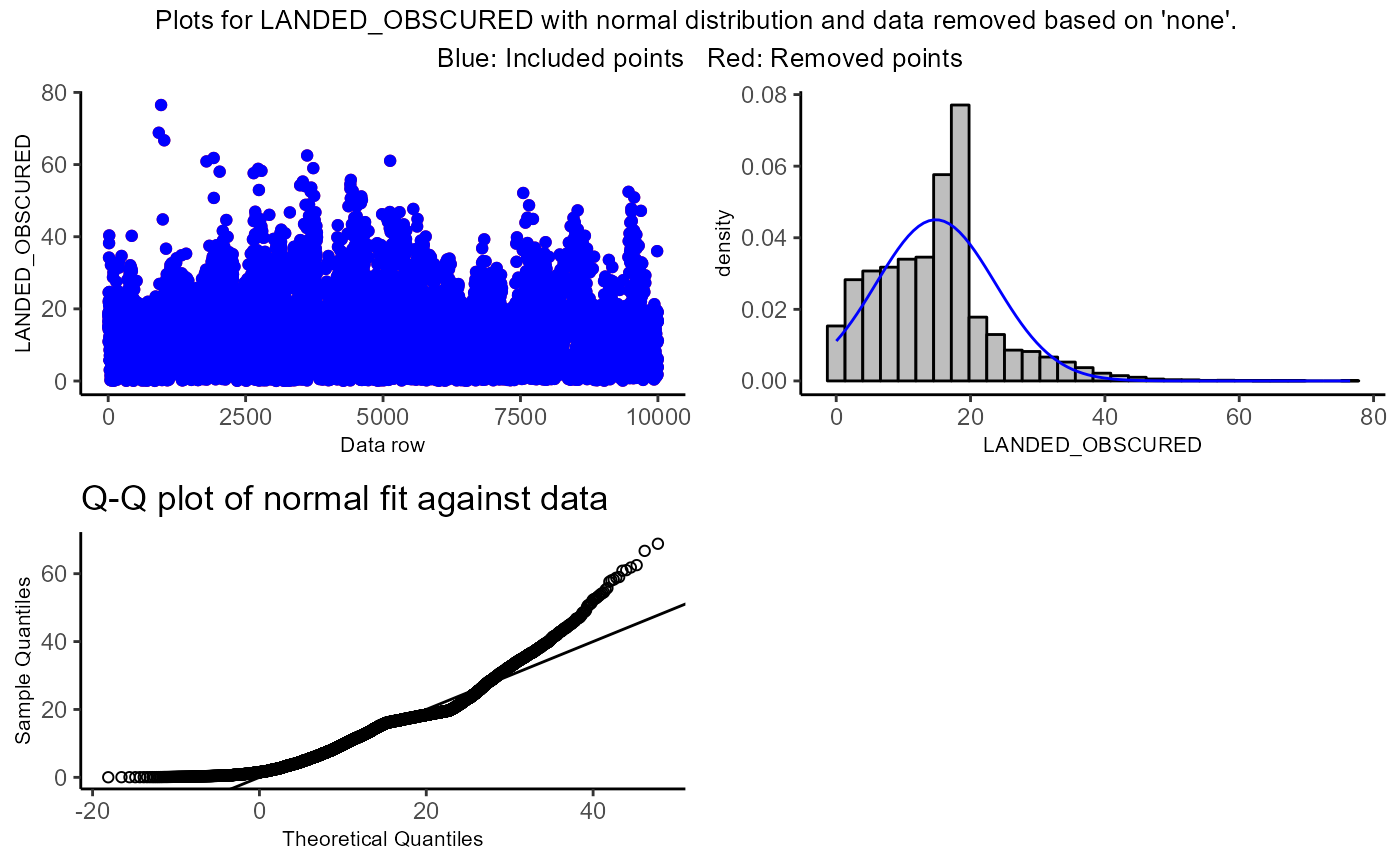

#> TableGrob (3 x 2) "arrange": 4 grobs
#>   z     cells    name                grob
#> 1 1 (2-2,1-1) arrange      gtable[layout]
#> 2 2 (2-2,2-2) arrange      gtable[layout]
#> 3 3 (3-3,1-1) arrange      gtable[layout]
#> 4 4 (1-1,1-2) arrange text[GRID.text.379]

outlier_plot(scallopMainDataTable, proj,
             x = "LANDED_OBSCURED", 
             dat.remove = "mean_3SD",
             x.dist = "normal",
             output.screen = TRUE)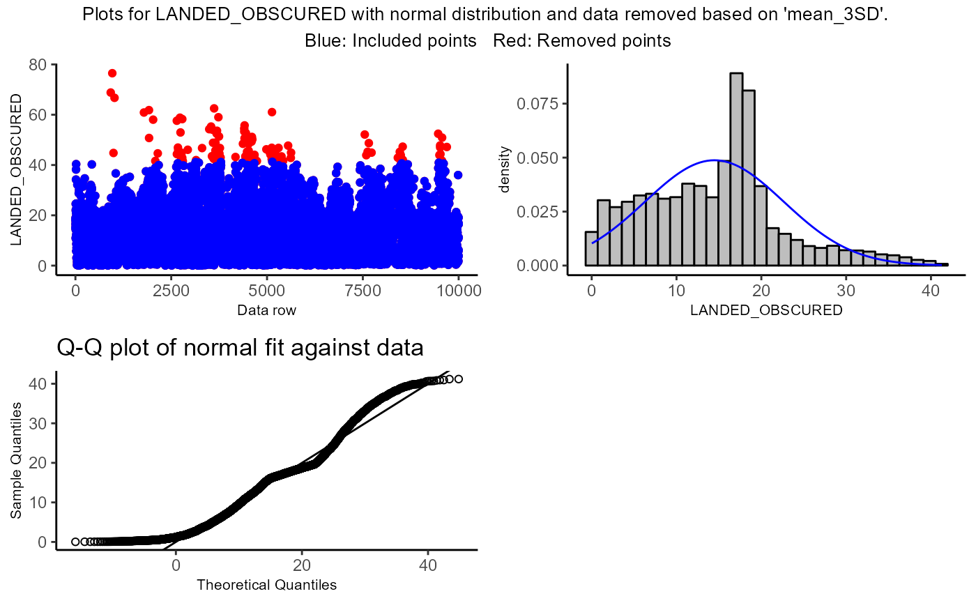

#> TableGrob (3 x 2) "arrange": 4 grobs
#>   z     cells    name                grob
#> 1 1 (2-2,1-1) arrange      gtable[layout]
#> 2 2 (2-2,2-2) arrange      gtable[layout]
#> 3 3 (3-3,1-1) arrange      gtable[layout]
#> 4 4 (1-1,1-2) arrange text[GRID.text.488]

Temporal Plots

temp_plot(scallopMainDataTable, proj,
          var.select = "LANDED_OBSCURED",
          len.fun = "percent",
          agg.fun = "sum",
          date.var = "DATE_TRIP",
          pages = "multi")
#> $scatter_plot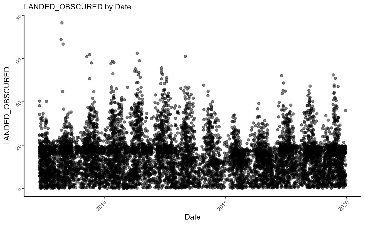

#> 
#> $unique_plot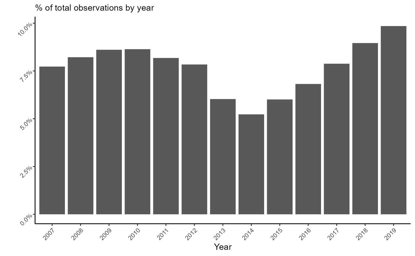

#> 
#> $agg_plot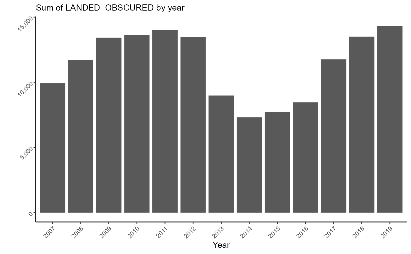

temp_plot(scallopMainDataTable, proj,
          var.select = "TRIP_LENGTH",
          len.fun = "percent",
          agg.fun = "sum",
          date.var = "DATE_TRIP",
          pages = "multi")
#> $scatter_plot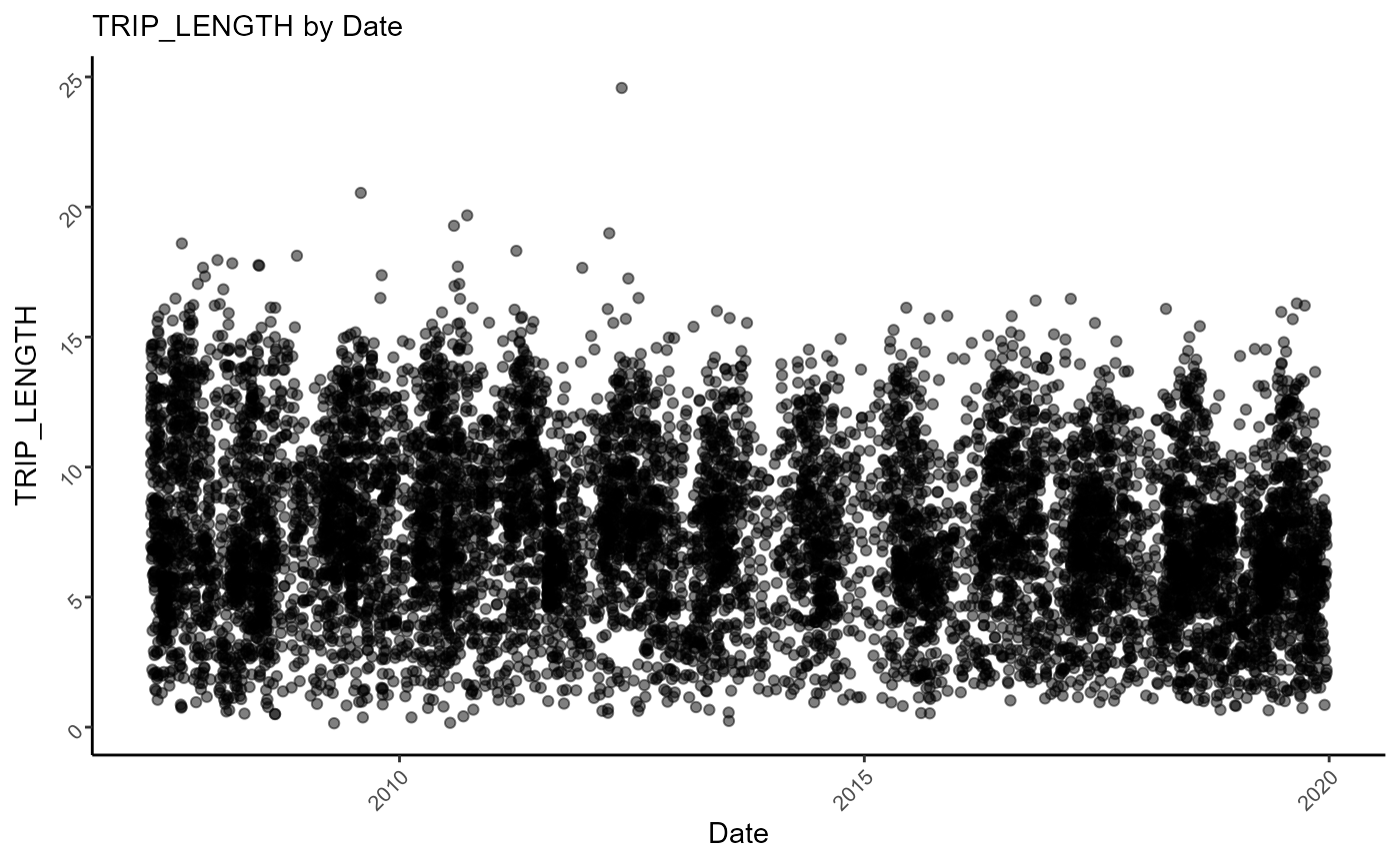

#> 
#> $unique_plot

#> 
#> $agg_plot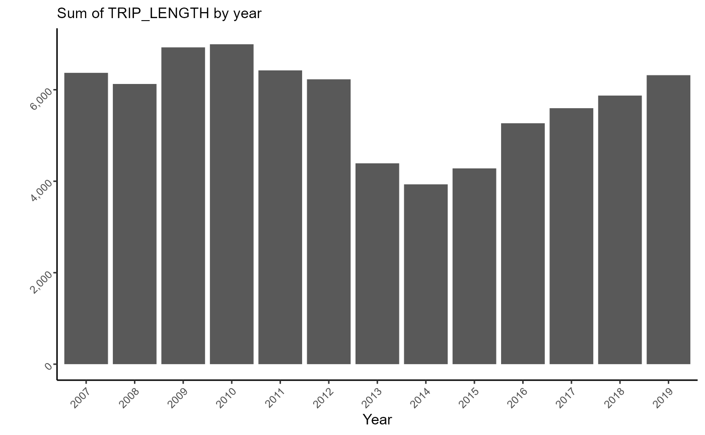

temp_plot(scallopMainDataTable, proj,
          var.select = "DOLLAR_OBSCURED",
          len.fun = "percent",
          agg.fun = "sum",
          date.var = "DATE_TRIP",
          pages = "multi")
#> $scatter_plot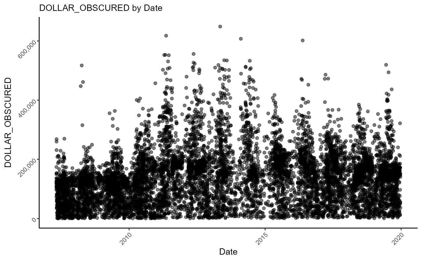

#> 
#> $unique_plot

#> 
#> $agg_plot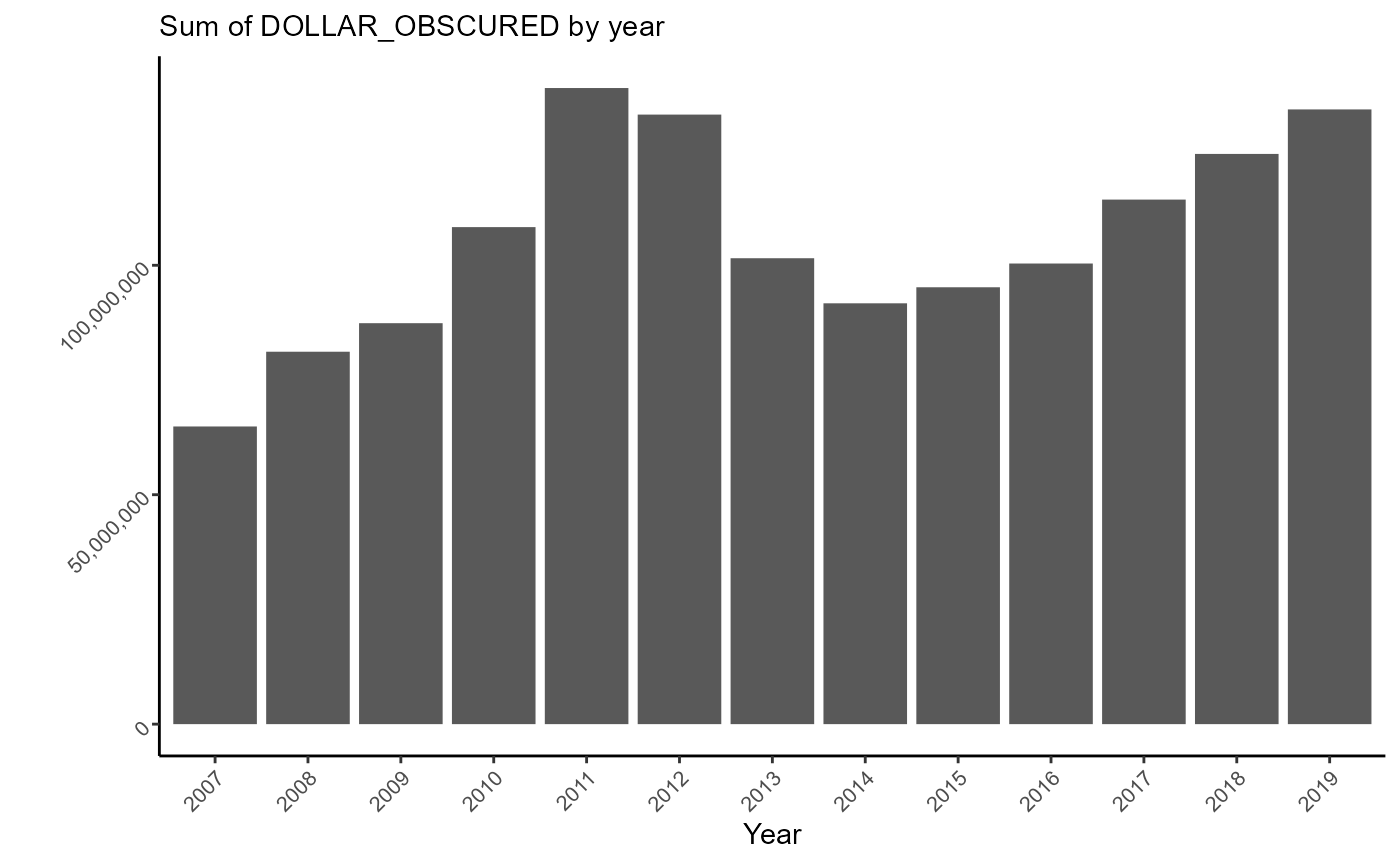

Scatter Plots

Trip length by meat catch.

xy_plot(scallopMainDataTable, proj,
        var1 = "TRIP_LENGTH", var2 = "LANDED_OBSCURED",
        regress = FALSE, alpha = .3)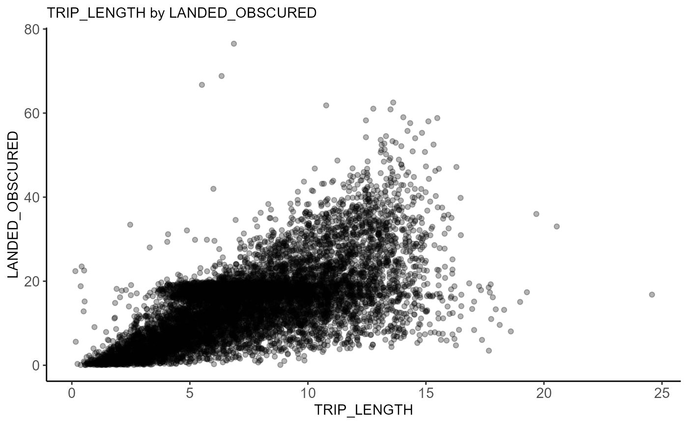

Trip length by revenue.

xy_plot(scallopMainDataTable, proj,
        var1 = "TRIP_LENGTH", var2 = "DOLLAR_OBSCURED",
        regress = FALSE, alpha = .3)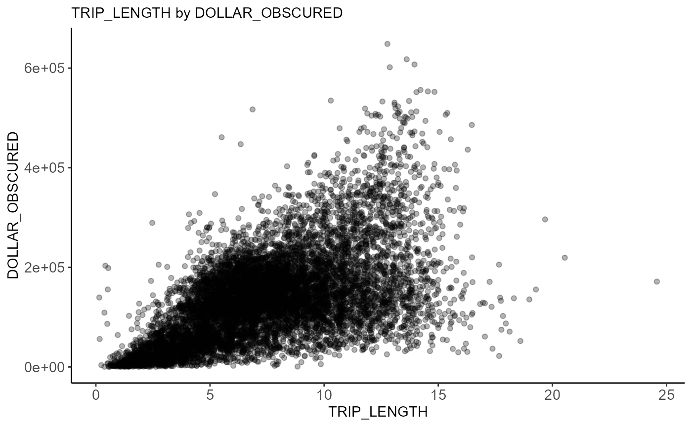

Trip length by trip cost (Winsor).

xy_plot(scallopMainDataTable, proj,
        var1 = "TRIP_LENGTH", var2 = "TRIP_COST_WINSOR_2020_DOL",
        regress = FALSE, alpha = .3)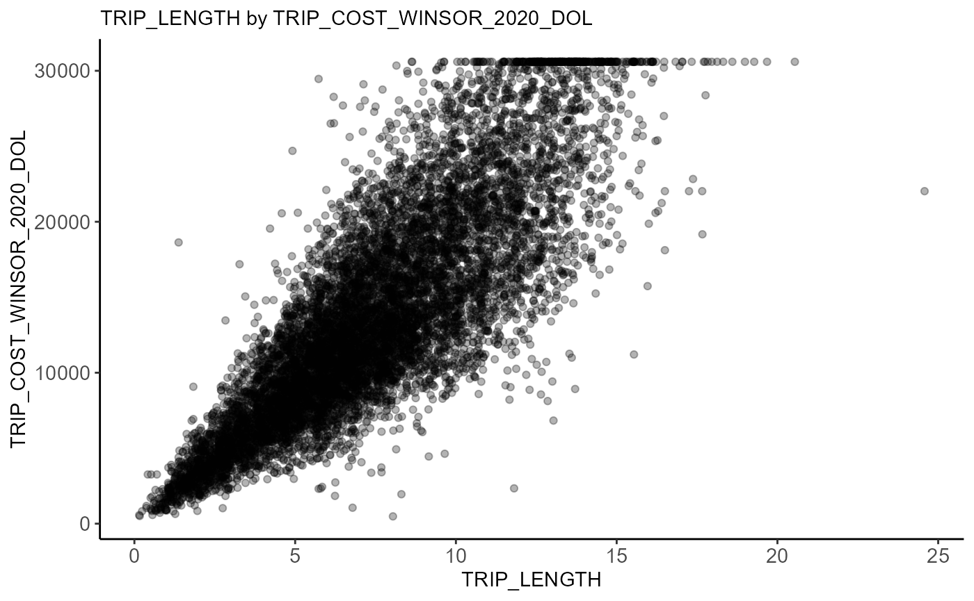

Correlation Matrix

corr_outs <-
  corr_out(scallopMainDataTable, proj,
           variables = "all",
           method = "pearson", 
           show_coef = FALSE)
#> Warning: No variance found in fleetAssignPlaceholder. Removed from correlation
#> test

corr_outs$plot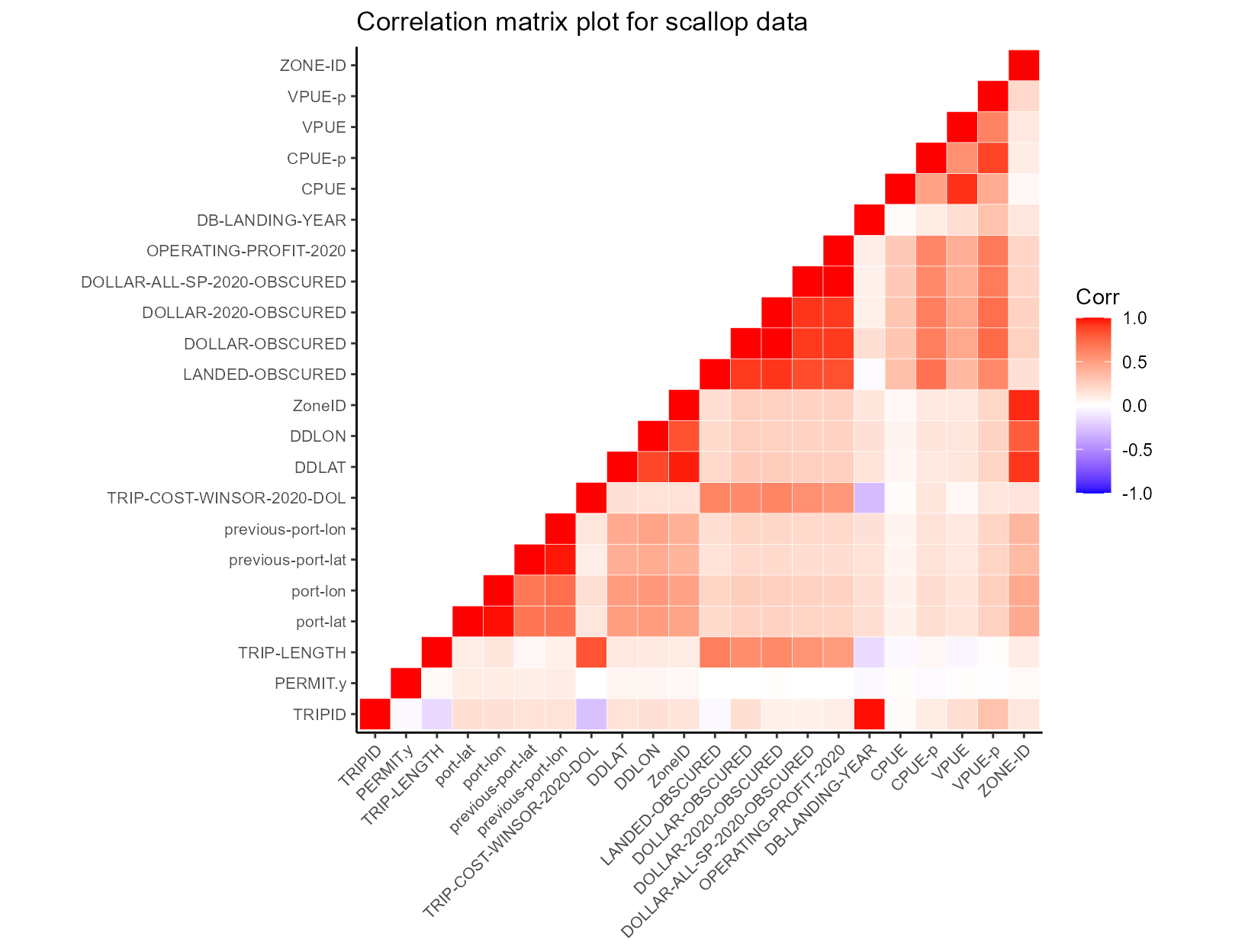

corr_outs$table %>% 
  pretty_tab_sb(width = "100%")

	TRIPID	PERMIT.y	TRIP-LENGTH	port-lat	port-lon	previous-port-lat	previous-port-lon	TRIP-COST-WINSOR-2020-DOL	DDLAT	DDLON	ZoneID	LANDED-OBSCURED	DOLLAR-OBSCURED	DOLLAR-2020-OBSCURED	DOLLAR-ALL-SP-2020-OBSCURED	OPERATING-PROFIT-2020	DB-LANDING-YEAR	CPUE	CPUE-p	VPUE	VPUE-p	ZONE-ID
TRIPID	1.00	-0.03	-0.16	0.17	0.16	0.15	0.15	-0.27	0.15	0.16	0.14	-0.03	0.17	0.08	0.07	0.09	0.99	0.02	0.10	0.17	0.32	0.13
PERMIT.y	-0.03	1.00	0.03	0.10	0.10	0.09	0.10	0.00	0.05	0.05	0.04	0.00	0.00	0.01	0.00	0.00	-0.03	0.01	-0.02	0.01	-0.01	0.03
TRIP-LENGTH	-0.16	0.03	1.00	0.09	0.13	0.04	0.08	0.83	0.12	0.11	0.10	0.65	0.58	0.60	0.55	0.51	-0.15	-0.03	0.04	-0.04	0.01	0.10
port-lat	0.17	0.10	0.09	1.00	0.99	0.69	0.70	0.13	0.50	0.51	0.47	0.19	0.24	0.23	0.22	0.22	0.17	0.07	0.17	0.14	0.24	0.44
port-lon	0.16	0.10	0.13	0.99	1.00	0.68	0.72	0.17	0.51	0.53	0.48	0.22	0.26	0.25	0.24	0.23	0.17	0.07	0.18	0.14	0.25	0.45
previous-port-lat	0.15	0.09	0.04	0.69	0.68	1.00	0.98	0.09	0.42	0.43	0.39	0.15	0.20	0.19	0.18	0.18	0.15	0.06	0.15	0.12	0.22	0.36
previous-port-lon	0.15	0.10	0.08	0.70	0.72	0.98	1.00	0.13	0.44	0.47	0.41	0.17	0.22	0.21	0.20	0.20	0.16	0.06	0.15	0.12	0.22	0.38
TRIP-COST-WINSOR-2020-DOL	-0.27	0.00	0.83	0.13	0.17	0.09	0.13	1.00	0.16	0.15	0.15	0.62	0.59	0.62	0.57	0.53	-0.29	0.02	0.13	0.04	0.13	0.14
DDLAT	0.15	0.05	0.12	0.50	0.51	0.42	0.44	0.16	1.00	0.87	0.97	0.20	0.27	0.26	0.25	0.25	0.14	0.05	0.12	0.13	0.22	0.92
DDLON	0.16	0.05	0.11	0.51	0.53	0.43	0.47	0.15	0.87	1.00	0.84	0.19	0.25	0.24	0.23	0.23	0.16	0.06	0.14	0.13	0.23	0.79
ZoneID	0.14	0.04	0.10	0.47	0.48	0.39	0.41	0.15	0.97	0.84	1.00	0.17	0.25	0.24	0.23	0.23	0.13	0.04	0.11	0.12	0.21	0.95
LANDED-OBSCURED	-0.03	0.00	0.65	0.19	0.22	0.15	0.17	0.62	0.20	0.19	0.17	1.00	0.91	0.92	0.85	0.84	-0.02	0.33	0.70	0.37	0.60	0.16
DOLLAR-OBSCURED	0.17	0.00	0.58	0.24	0.26	0.20	0.22	0.59	0.27	0.25	0.25	0.91	1.00	1.00	0.91	0.91	0.17	0.30	0.65	0.45	0.74	0.24
DOLLAR-2020-OBSCURED	0.08	0.01	0.60	0.23	0.25	0.19	0.21	0.62	0.26	0.24	0.24	0.92	1.00	1.00	0.92	0.91	0.08	0.30	0.65	0.45	0.72	0.23
DOLLAR-ALL-SP-2020-OBSCURED	0.07	0.00	0.55	0.22	0.24	0.18	0.20	0.57	0.25	0.23	0.23	0.85	0.91	0.92	1.00	1.00	0.07	0.28	0.60	0.41	0.66	0.22
OPERATING-PROFIT-2020	0.09	0.00	0.51	0.22	0.23	0.18	0.20	0.53	0.25	0.23	0.23	0.84	0.91	0.91	1.00	1.00	0.09	0.28	0.61	0.42	0.67	0.22
DB-LANDING-YEAR	0.99	-0.03	-0.15	0.17	0.17	0.15	0.16	-0.29	0.14	0.16	0.13	-0.02	0.17	0.08	0.07	0.09	1.00	0.02	0.10	0.17	0.32	0.13
CPUE	0.02	0.01	-0.03	0.07	0.07	0.06	0.06	0.02	0.05	0.06	0.04	0.33	0.30	0.30	0.28	0.28	0.02	1.00	0.48	0.93	0.43	0.04
CPUE-p	0.10	-0.02	0.04	0.17	0.18	0.15	0.15	0.13	0.12	0.14	0.11	0.70	0.65	0.65	0.60	0.61	0.10	0.48	1.00	0.57	0.88	0.10
VPUE	0.17	0.01	-0.04	0.14	0.14	0.12	0.12	0.04	0.13	0.13	0.12	0.37	0.45	0.45	0.41	0.42	0.17	0.93	0.57	1.00	0.63	0.12
VPUE-p	0.32	-0.01	0.01	0.24	0.25	0.22	0.22	0.13	0.22	0.23	0.21	0.60	0.74	0.72	0.66	0.67	0.32	0.43	0.88	0.63	1.00	0.20
ZONE-ID	0.13	0.03	0.10	0.44	0.45	0.36	0.38	0.14	0.92	0.79	0.95	0.16	0.24	0.23	0.22	0.22	0.13	0.04	0.10	0.12	0.20	1.00

Active Vessels

vessel count by year.

ves_out <- 
  vessel_count(scallopMainDataTable, proj,
               v_id = "PERMIT.y",
               date = "DATE_TRIP",
               period = "year", type = "line")
#> Joining with `by = join_by(DATE_TRIP)`
#> Warning: Setting row names on a tibble is deprecated.

ves_out$table %>% pretty_tab()

year	PERMIT.y
2007	98
2008	96
2009	101
2010	100
2011	100
2012	98
2013	95
2014	96
2015	90
2016	92
2017	97
2018	98
2019	98

ves_out$plot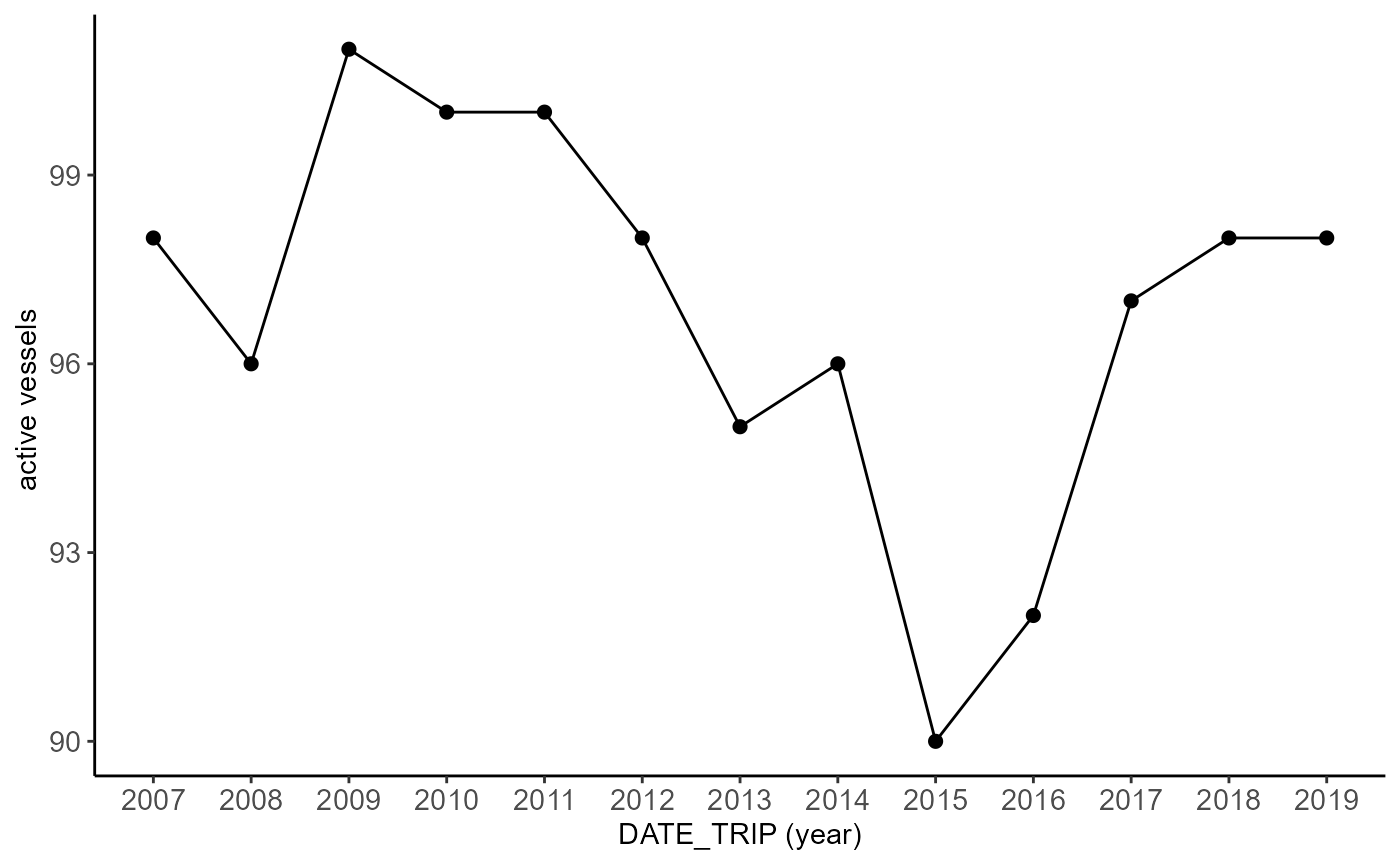 

vessel count by fleet.

ves_out <- 
  vessel_count(scallopMainDataTable, proj,
               v_id = "PERMIT.y",
               group = "fleet",
               output = "table")
#> Joining with `by = join_by(fleet)`
#> Warning: Setting row names on a tibble is deprecated.

ves_out$table %>% pretty_tab()
#> Warning: Unknown or uninitialised column: `table`.

ves_out$plot 
#> Warning: Unknown or uninitialised column: `plot`.
#> NULL

vessel count by year and fleet.

ves_out <- 
  vessel_count(scallopMainDataTable, proj,
               v_id = "PERMIT.y",
               group = "fleet",
               date = "DATE_TRIP",
               period = "year", type = "line")
#> Joining with `by = join_by(fleet, DATE_TRIP)`
#> Warning: Setting row names on a tibble is deprecated.

ves_out$table %>% 
  pretty_lab(cols = "PERMIT.y") %>% 
  pretty_tab_sb(width = "40%")

year	fleet	PERMIT.y
2007	Access Area	94
2007	Days at Sea	91
2008	Access Area	93
2008	Days at Sea	89
2009	Access Area	100
2009	Days at Sea	99
2010	Access Area	97
2010	Days at Sea	95
2011	Access Area	98
2011	Days at Sea	92
2012	Access Area	97
2012	Days at Sea	95
2013	Access Area	91
2013	Days at Sea	89
2014	Access Area	89
2014	Days at Sea	91
2015	Access Area	87
2015	Days at Sea	85
2016	Access Area	91
2016	Days at Sea	86
2017	Access Area	97
2017	Days at Sea	86
2018	Access Area	98
2018	Days at Sea	84
2019	Access Area	98
2019	Days at Sea	80

ves_out$plot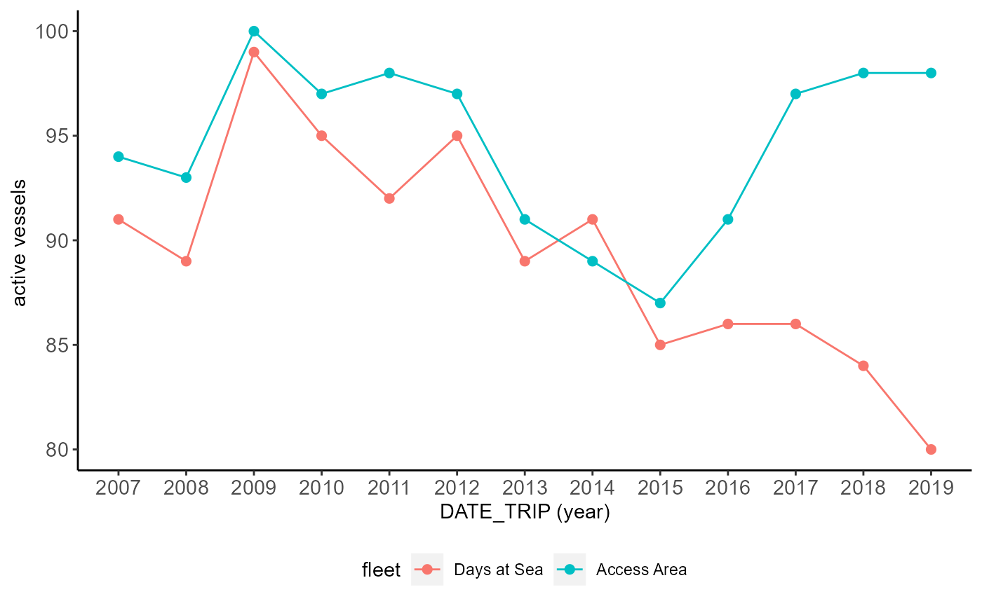 

vessel count by gearcode.

ves_out <- 
  vessel_count(scallopMainDataTable, proj,
               v_id = "PERMIT.y",
               group = "GEARCODE", tran = "log")
#> Joining with `by = join_by(GEARCODE)`
#> Warning: Setting row names on a tibble is deprecated.

ves_out$table %>% 
  pretty_lab() %>% 
  pretty_tab()

GEARCODE	PERMIT.y
DREDGE	130
OTHER	1
TRAWL-BOTTOM	5

ves_out$plot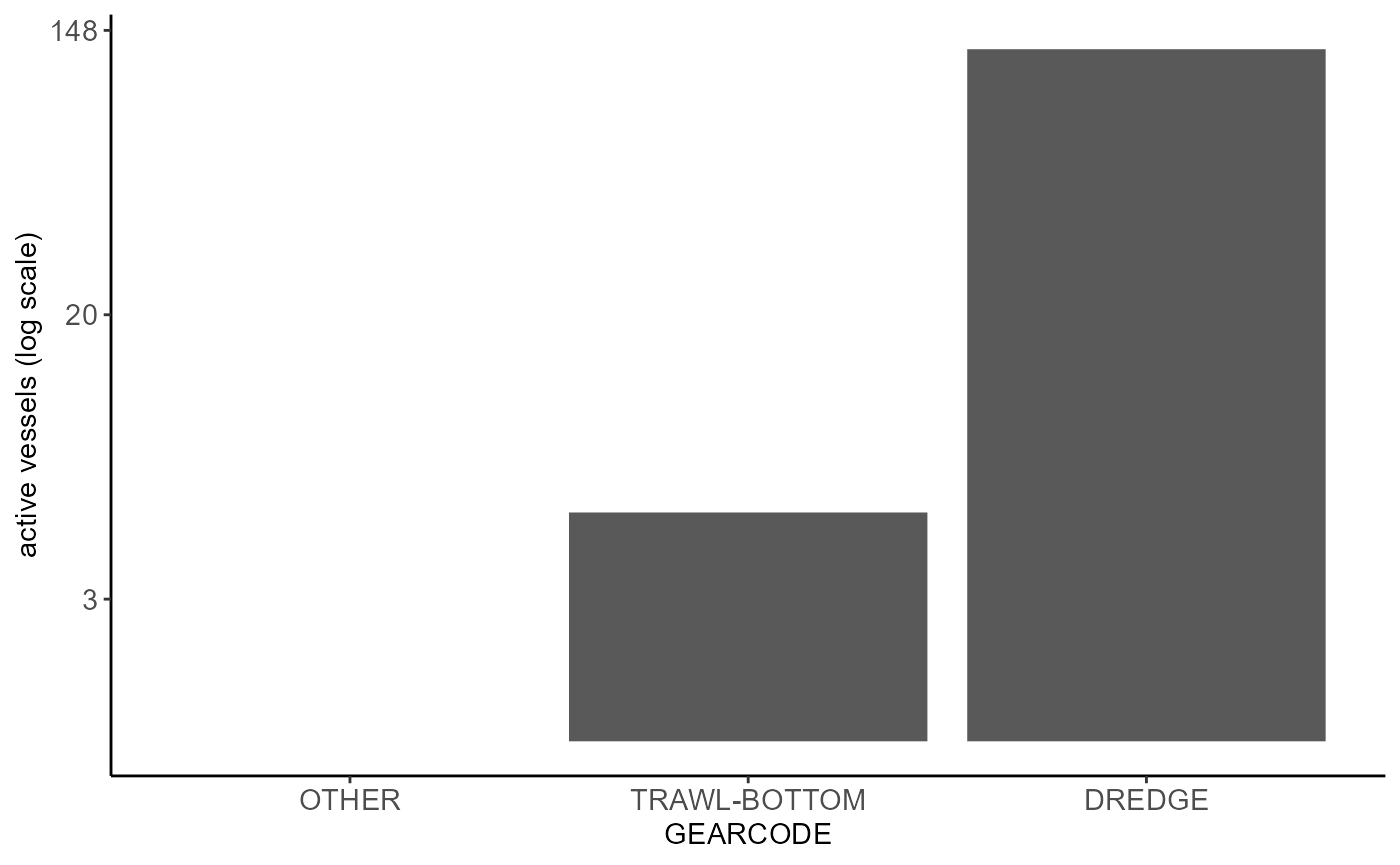

Catch

Total meat catch by year.

catch_out <- 
species_catch(scallopMainDataTable, proj,
              species = "LANDED_OBSCURED",
              date = "DATE_TRIP", 
              period = "year",
              fun = "sum",
              type = "line", format_lab = "decimal")
#> Joining with `by = join_by(DATE_TRIP)`

catch_out$table %>% 
  pretty_lab(cols = "LANDED_OBSCURED") %>%
  pretty_tab()

year	LANDED_OBSCURED
2007	9,931.51
2008	11,702.12
2009	13,420.05
2010	13,637.72
2011	13,996.77
2012	13,476.78
2013	8,982.47
2014	7,316.64
2015	7,706.52
2016	8,464.29
2017	11,756.92
2018	13,500.97
2019	14,328.6

catch_out$plot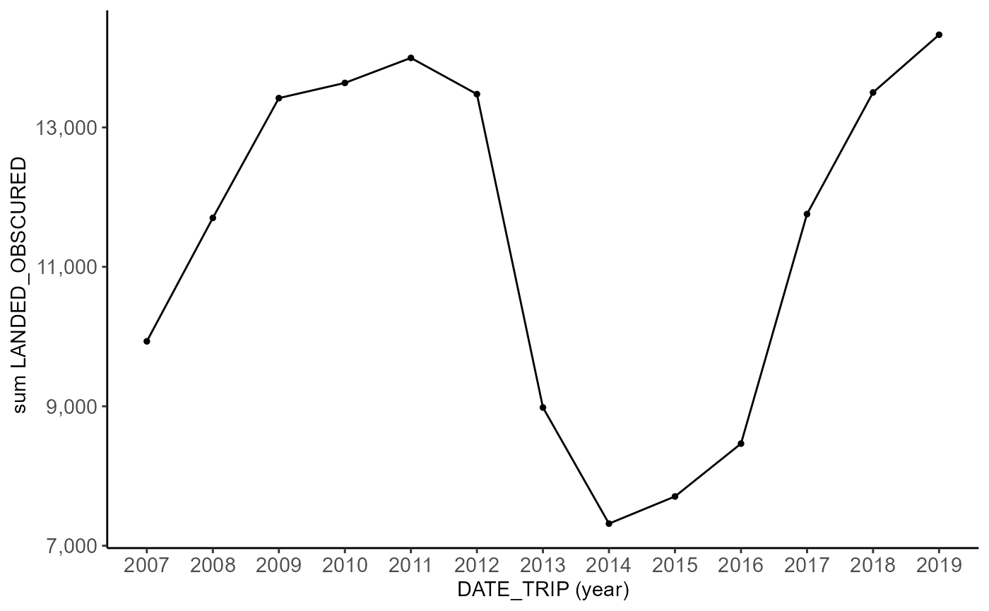

Total meat catch by fleet.

catch_out <- 
  species_catch(scallopMainDataTable, proj,
                species = "LANDED_OBSCURED",
                group = "fleet",
                fun = "sum",
                type = "bar", format_lab = "decimal")
#> Joining with `by = join_by(fleet)`

catch_out$table %>% 
  pretty_lab(cols = "LANDED_OBSCURED") %>%
  pretty_tab()

fleet	LANDED_OBSCURED
Access Area	73,842.46
Days at Sea	74,378.91

catch_out$plot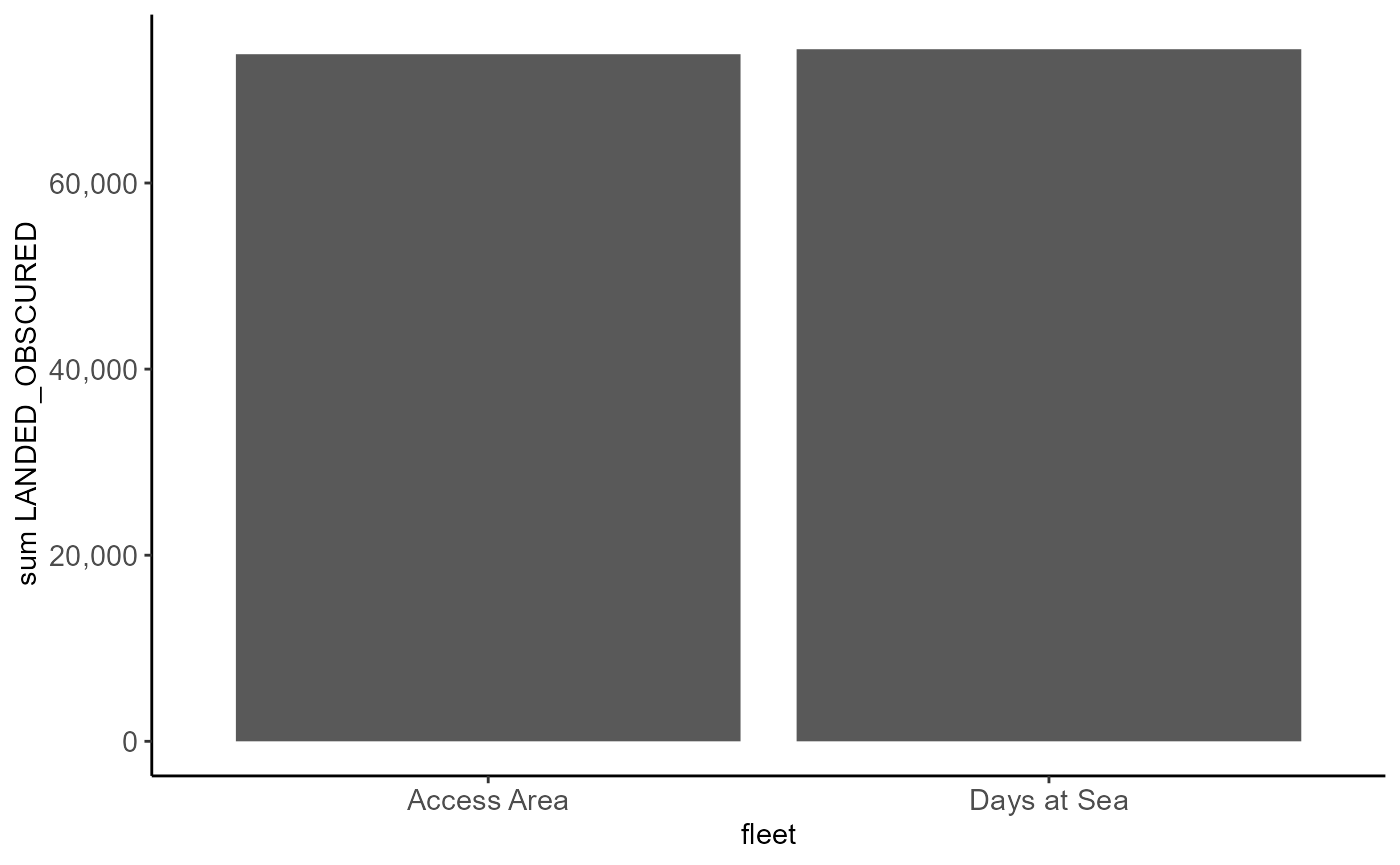

Total meat catch by year and fleet.

catch_out <- 
  species_catch(scallopMainDataTable, proj,
                species = "LANDED_OBSCURED",
                date = "DATE_TRIP", 
                period = "year",
                group = "fleet",
                fun = "sum",
                type = "line", format_lab = "decimal")
#> Joining with `by = join_by(fleet, DATE_TRIP)`

catch_out$table %>% 
  pretty_lab(cols = "LANDED_OBSCURED") %>%
  pretty_tab_sb(width = "40%")

year	fleet	LANDED_OBSCURED
2007	Access Area	5,706.6
2007	Days at Sea	4,224.91
2008	Access Area	7,216.21
2008	Days at Sea	4,485.92
2009	Access Area	6,843.84
2009	Days at Sea	6,576.2
2010	Access Area	5,520.37
2010	Days at Sea	8,117.35
2011	Access Area	6,366.48
2011	Days at Sea	7,630.29
2012	Access Area	5,680.09
2012	Days at Sea	7,796.69
2013	Access Area	2,141.4
2013	Days at Sea	6,841.07
2014	Access Area	1,693.68
2014	Days at Sea	5,622.95
2015	Access Area	3,921.89
2015	Days at Sea	3,784.62
2016	Access Area	3,928.59
2016	Days at Sea	4,535.7
2017	Access Area	6,112.54
2017	Days at Sea	5,644.38
2018	Access Area	8,712.77
2018	Days at Sea	4,788.2
2019	Access Area	9,998
2019	Days at Sea	4,330.6

catch_out$plot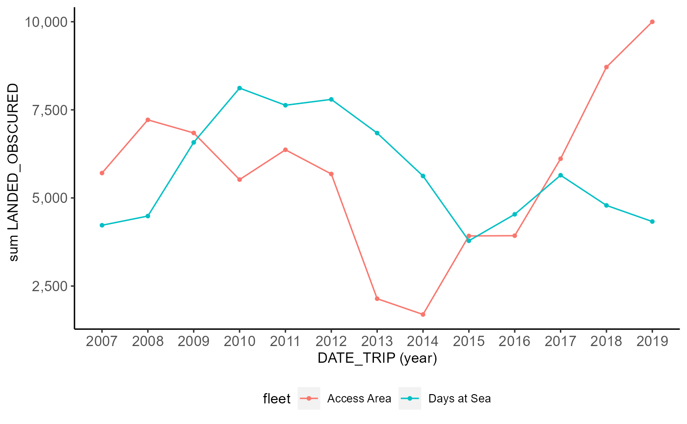

CPUE

Average CPUE by year.

cpue_out <- 
  species_catch(scallopMainDataTable, proj,
                species = "CPUE",
                date = "DATE_TRIP", 
                period = "year",
                fun = "mean", type = "line")
#> Joining with `by = join_by(DATE_TRIP)`

cpue_out$table %>% 
  pretty_lab(cols = "CPUE") %>%
  pretty_tab()

year	CPUE
2007	1.71
2008	2.14
2009	2.11
2010	1.98
2011	2.16
2012	2.06
2013	1.96
2014	1.78
2015	1.84
2016	1.54
2017	2.03
2018	2.25
2019	2.24

cpue_out$plot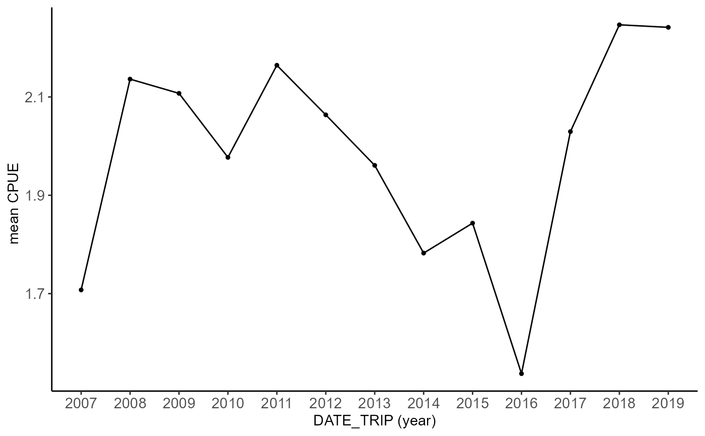

Average CPUE by year and fleet.

cpue_out <- 
  species_catch(scallopMainDataTable, proj,
                species = "CPUE",
                date = "DATE_TRIP", 
                period = "year",
                group = "fleet",
                fun = "mean", type = "line")
#> Joining with `by = join_by(fleet, DATE_TRIP)`

cpue_out$table %>% 
  pretty_lab(cols = "CPUE") %>%
  pretty_tab_sb(width = "40%")

year	fleet	CPUE
2007	Access Area	2.13
2007	Days at Sea	1.19
2008	Access Area	2.76
2008	Days at Sea	1.29
2009	Access Area	2.05
2009	Days at Sea	2.18
2010	Access Area	1.71
2010	Days at Sea	2.28
2011	Access Area	1.89
2011	Days at Sea	2.6
2012	Access Area	1.72
2012	Days at Sea	2.49
2013	Access Area	1.24
2013	Days at Sea	2.45
2014	Access Area	1.64
2014	Days at Sea	1.85
2015	Access Area	2.31
2015	Days at Sea	1.36
2016	Access Area	1.53
2016	Days at Sea	1.55
2017	Access Area	2
2017	Days at Sea	2.07
2018	Access Area	2.31
2018	Days at Sea	2.08
2019	Access Area	2.28
2019	Days at Sea	2.12

cpue_out$plot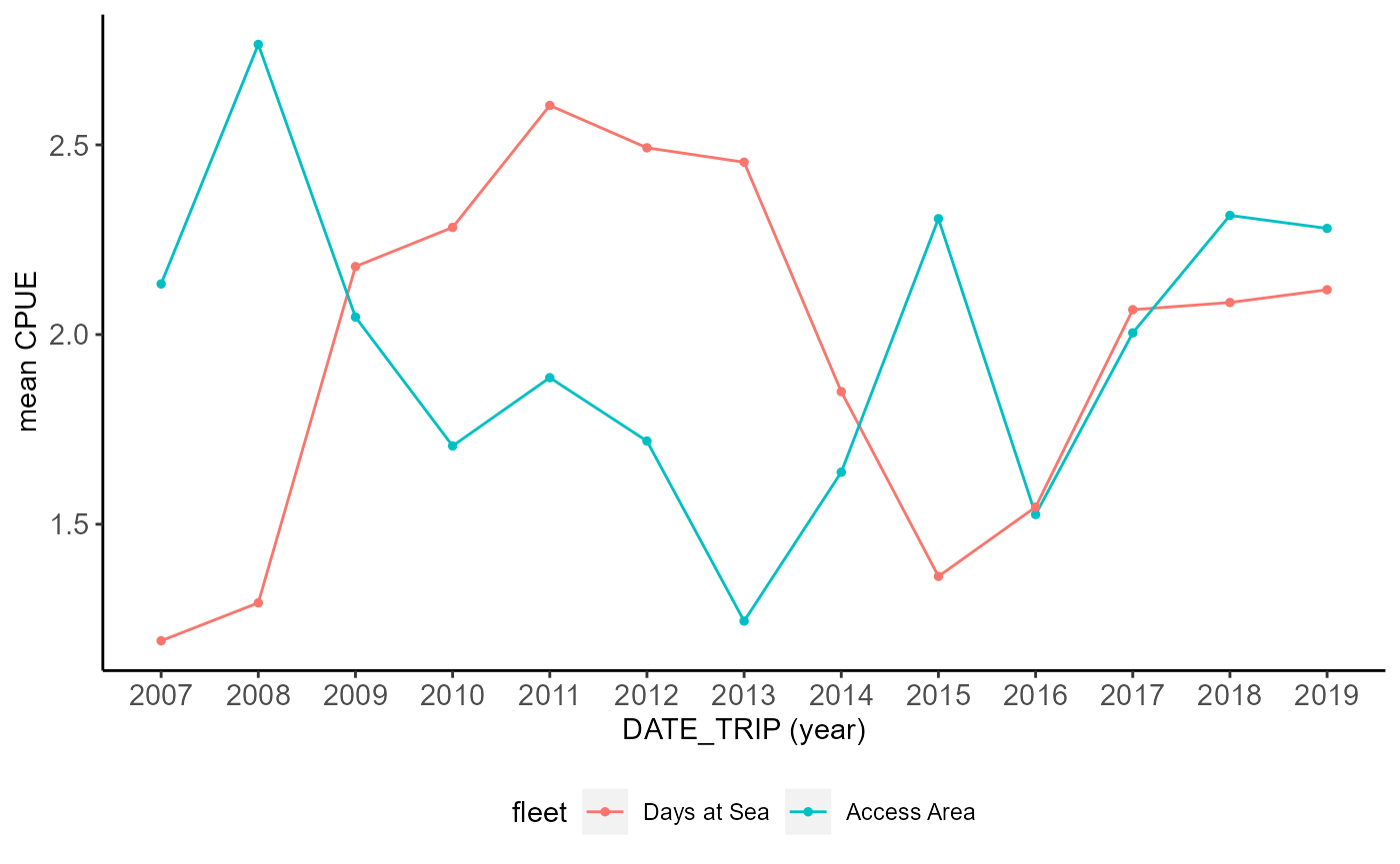

VPUE

Average VPUE by year.

vpue_out <- 
  species_catch(scallopMainDataTable, proj,
                species = "VPUE",
                date = "DATE_TRIP", 
                period = "year",
                fun = "mean", type = "line")
#> Joining with `by = join_by(DATE_TRIP)`

vpue_out$table %>% 
  pretty_lab(cols = "VPUE") %>%
  pretty_tab()

year	VPUE
2007	11,216.91
2008	14,807.41
2009	13,694.33
2010	16,039.3
2011	21,511.01
2012	20,405.14
2013	22,201.91
2014	22,354.77
2015	22,822.66
2016	18,180.2
2017	20,256.65
2018	20,940.58
2019	21,062.97

vpue_out$plot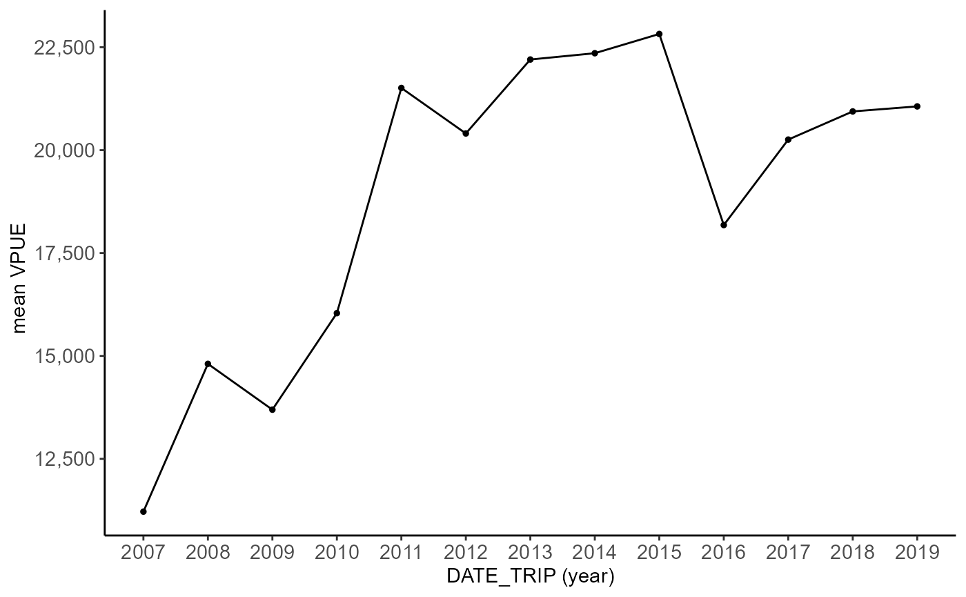

Average VPUE by year and fleet.

vpue_out <- 
  species_catch(scallopMainDataTable, proj,
                species = "VPUE",
                date = "DATE_TRIP", 
                period = "year",
                group = "fleet",
                fun = "mean", type = "line")
#> Joining with `by = join_by(fleet, DATE_TRIP)`

vpue_out$table %>% 
  pretty_lab(cols = "VPUE") %>%
  pretty_tab_sb(width = "40%")

year	fleet	VPUE
2007	Access Area	14,054.84
2007	Days at Sea	7,787.08
2008	Access Area	19,176.6
2008	Days at Sea	8,944.48
2009	Access Area	13,539.66
2009	Days at Sea	13,854.48
2010	Access Area	14,678.53
2010	Days at Sea	17,574.35
2011	Access Area	18,967.12
2011	Days at Sea	25,531.48
2012	Access Area	17,096.89
2012	Days at Sea	24,522.17
2013	Access Area	14,437.7
2013	Days at Sea	27,552.04
2014	Access Area	20,732.08
2014	Days at Sea	23,097.61
2015	Access Area	28,535.36
2015	Days at Sea	16,879.25
2016	Access Area	17,909.21
2016	Days at Sea	18,421.18
2017	Access Area	21,327.81
2017	Days at Sea	18,722.65
2018	Access Area	21,660.23
2018	Days at Sea	19,218.95
2019	Access Area	20,920.47
2019	Days at Sea	21,404.03

vpue_out$plot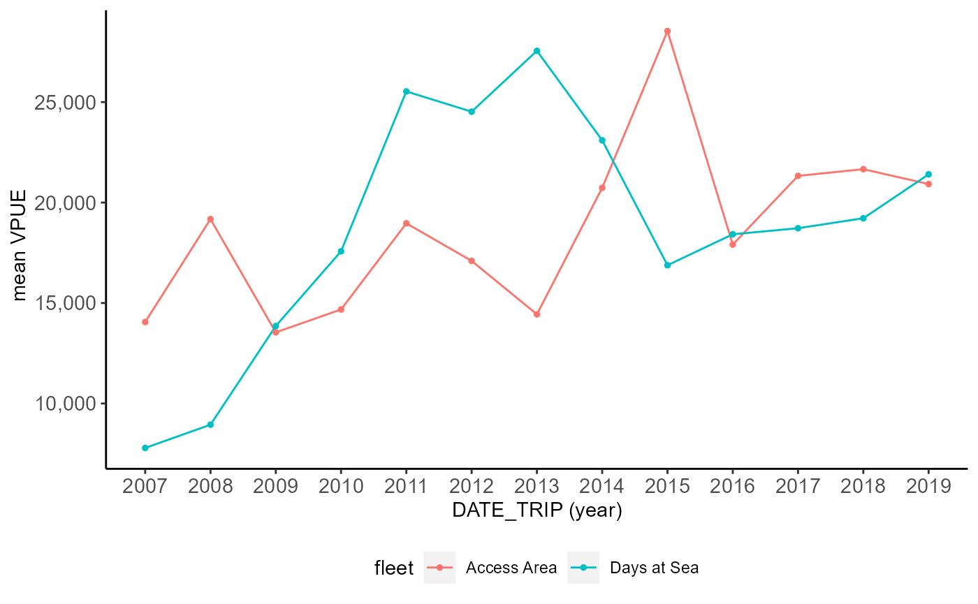

Average VPUE by gearcode.

vpue_out <- 
  species_catch(scallopMainDataTable, proj,
                species = "VPUE",
                group = "GEARCODE",
                fun = "mean", type = "line")
#> Joining with `by = join_by(GEARCODE)`

vpue_out$table %>% 
pretty_lab() %>%
  pretty_tab()

GEARCODE	VPUE
DREDGE	18,745.93
OTHER	14,069.03
TRAWL-BOTTOM	10,273.8

vpue_out$plot + angled_theme()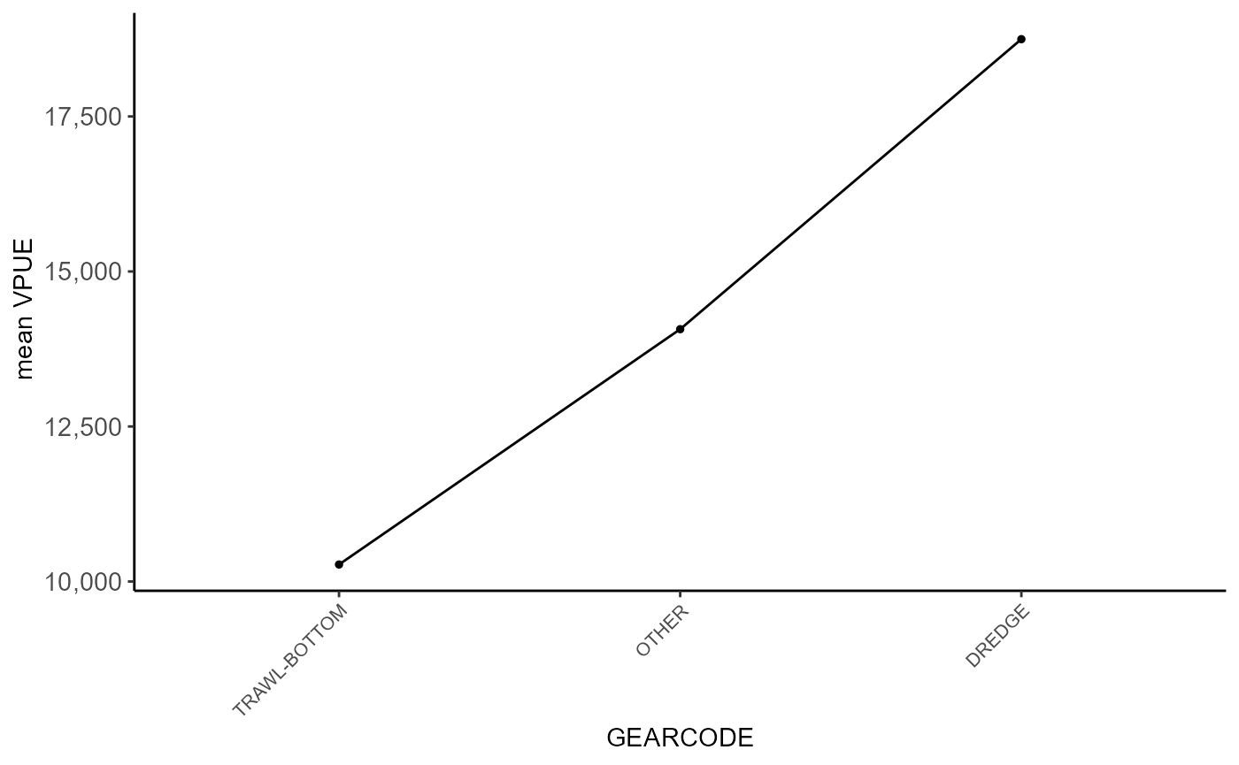

Distributions

LANDED_OBSCURED

KDE, ECDF, and CDF of meat catch.

density_plot(scallopMainDataTable, proj,
             var = "LANDED_OBSCURED", 
             type = "all", tran = "log")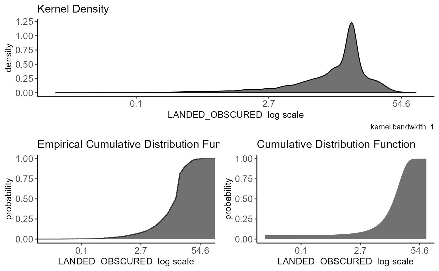

KDE, ECDF, and CDF of meat catch by fleet.

density_plot(scallopMainDataTable, proj,
             var = "LANDED_OBSCURED",
             group = "fleet", position = "stack", 
             type = "all", tran = "log", pages = "multi")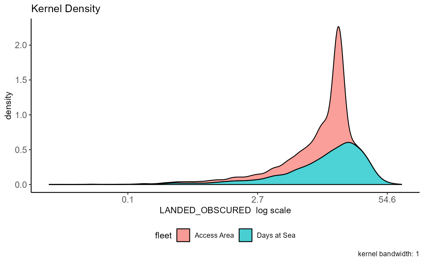

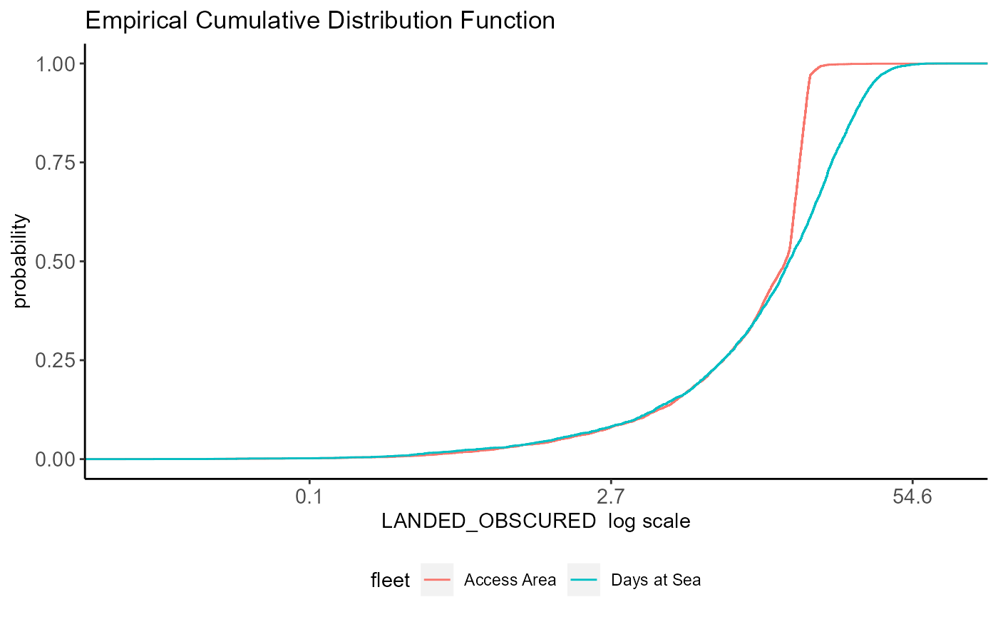
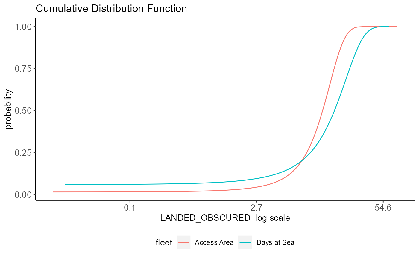
KDE of meat catch by year.

density_plot(scallopMainDataTable, proj,
             var = "LANDED_OBSCURED", 
             facet_by = "DB_LANDING_YEAR",
             filter_by = "DB_LANDING_YEAR",
             filter_value = 2007:2013,
             type = "kde", bw = 1.5, 
             tran = "log", scale = "free_y") + 
  angled_theme()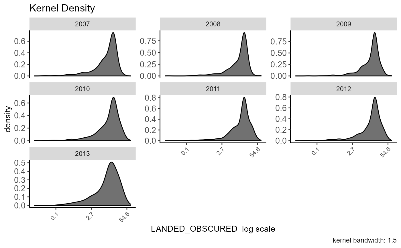

density_plot(scallopMainDataTable, proj,
             var = "LANDED_OBSCURED", 
             facet_by = "DB_LANDING_YEAR",
             filter_by = "DB_LANDING_YEAR",
             filter_value = 2014:2019,
             type = "kde", bw = 1.5, 
             tran = "log", scale = "free_y") + 
  angled_theme()